Two-dimensional random variable. Discrete two-dimensional random variables Find the distribution of a two-dimensional random variable

Let a two-dimensional random variable $(X,Y)$ be given.

Definition 1

The distribution law of a two-dimensional random variable $(X,Y)$ is the set of possible pairs of numbers $(x_i,\ y_j)$ (where $x_i \epsilon X,\ y_j \epsilon Y$) and their probabilities $p_(ij)$ .

Most often, the distribution law of a two-dimensional random variable is written in the form of a table (Table 1).

Figure 1. Law of distribution of a two-dimensional random variable.

Let's remember now theorem on the addition of probabilities of independent events.

Theorem 1

The probability of the sum of a finite number of independent events $(\ A)_1$, $(\ A)_2$, ... ,$\ (\ A)_n$ is calculated by the formula:

Using this formula, one can obtain distribution laws for each component of a two-dimensional random variable, that is:

From here it will follow that the sum of all probabilities of a two-dimensional system has the following form:

Let us consider in detail (step by step) the problem associated with the concept of the distribution law of a two-dimensional random variable.

Example 1

The distribution law of a two-dimensional random variable is given by the following table:

Figure 2.

Find the laws of distribution of random variables $X,\ Y$, $X+Y$ and check in each case that the total sum of probabilities is equal to one.

Let us first find the distribution of the random variable $X$. The random variable $X$ can take the values $x_1=2,$ $x_2=3$, $x_3=5$. To find the distribution, we will use Theorem 1.

Let us first find the sum of probabilities $x_1$ as follows:

Figure 3

Similarly, we find $P\left(x_2\right)$ and $P\left(x_3\right)$:

\ \

Figure 4

Let us now find the distribution of the random variable $Y$. The random variable $Y$ can take the values $x_1=1,$ $x_2=3$, $x_3=4$. To find the distribution, we will use Theorem 1.

Let us first find the sum of probabilities $y_1$ as follows:

Figure 5

Similarly, we find $P\left(y_2\right)$ and $P\left(y_3\right)$:

\ \

Hence, the law of distribution of the quantity $X$ has the following form:

Figure 6

Let's check the fulfillment of the equality of the total sum of probabilities:

It remains to find the law of distribution of the random variable $X+Y$.

Let's designate it for convenience through $Z$: $Z=X+Y$.

First, let's find what values can take given value. To do this, we will pairwise add the values of $X$ and $Y$. We get the following values: 3, 4, 6, 5, 6, 8, 6, 7, 9. Now, discarding the matched values, we get that the random variable $X+Y$ can take the values $z_1=3,\ z_2=4 ,\ z_3=5,\ z_4=6,\ z_5=7,\ z_6=8,\ z_7=9.\ $

First, let's find $P(z_1)$. Since the value of $z_1$ is single, it is found as follows:

Figure 7

All probabilities are found similarly, except for $P(z_4)$:

Let us now find $P(z_4)$ as follows:

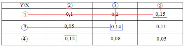
Figure 8

Hence, the distribution law for $Z$ has the following form:

Figure 9

Let's check the fulfillment of the equality of the total sum of probabilities:

two-dimensional discrete distribution random

Often the result of the experiment is described by several random variables: . For example, the weather in a given place at a certain time of the day can be characterized by the following random variables: X 1 - temperature, X 2 - pressure, X 3 - air humidity, X 4 - wind speed.

In this case, one speaks of a multidimensional random variable or a system of random variables.

Consider a two-dimensional random variable whose possible values are pairs of numbers. Geometrically, a two-dimensional random variable can be interpreted as a random point on a plane.

If the components X and Y are discrete random variables, then is a discrete two-dimensional random variable, and if X and Y are continuous, then is a continuous two-dimensional random variable.

The law of probability distribution of a two-dimensional random variable is the correspondence between possible values and their probabilities.

The distribution law of a two-dimensional discrete random variable can be given in the form of a double-entry table (see Table 6.1), where is the probability that the component X took on the meaning x i, and the component Y- meaning y j .

Table 6.1.1.

	y 1	y 2	y j	y m
x 1	p 11	p 12	p 1j	p 1m
x 2	p 21	p 22	p 2j	p 2m

x i	p i1	p i2	p ij	p im

x n	p n1	p n2	p nj	p nm

Since events make up a complete group of pairwise incompatible events, the sum of probabilities is equal to 1, i.e.

From table 6.1 you can find the laws of distribution of one-dimensional components X and Y.

Example 6.1.1 . Find the laws of distribution of components X and Y, if the distribution of a two-dimensional random variable is given in the form of table 6.1.2.

Table 6.1.2.

If we fix the value of one of the arguments, for example, then the resulting distribution of the quantity X is called a conditional distribution. The conditional distribution is defined similarly Y.

Example 6.1.2 . According to the distribution of a two-dimensional random variable given in Table. 6.1.2, find: a) the conditional distribution law of the component X given that; b) conditional distribution law Y provided that.

Decision. Conditional probabilities of components X and Y calculated by formulas

Conditional distribution law X condition has the form

Control: .

The distribution law of a two-dimensional random variable can be given as distribution functions, which determines for each pair of numbers the probability that X takes on a value less than X, and wherein Y takes on a value less than y:

Geometrically, the function means the probability of a random point falling into an infinite square with a vertex at the point (Fig. 6.1.1).

Let's note the properties.

1. The range of the function - , i.e. .
2. Function - non-decreasing function for each argument.
3. There are limiting relations:

At , the distribution function of the system becomes equal to the distribution function of the component X, i.e. .

Likewise, .

Knowing, you can find the probability of a random point falling within the rectangle ABCD.

Namely,

Example 6.1.3. Bivariate discrete random variable defined by distribution table

Find the distribution function.

Decision. Value in case of discrete components X and Y is found by summing all probabilities with indices i and j, for which, . Then, if and, then (the events and are impossible). Similarly, we get:

if and then;

if and then.

The results obtained are presented in the form of a table (6.1.3) of values:

For two-dimensional continuous random variable, the concept of probability density is introduced

The geometric probability density is a distribution surface in space

A two-dimensional probability density has the following properties:

3. The distribution function can be expressed in terms of the formula

4. The probability of hitting a continuous random variable in the area is equal to

5. In accordance with property (4) of the function, the formulas take place:

Example 6.1.4. The distribution function of a two-dimensional random variable is given

Definition. If two random variables are given on the same space of elementary events X and Y, then they say that it is given two-dimensional random variable (X,Y) .

Example. The machine stamps steel tiles. Length controlled X and width Y. − two-dimensional SW.

SW X and Y have their own distribution functions and other characteristics.

Definition. The distribution function of a two-dimensional random variable (X, Y) is called a function.

Definition. The distribution law of a discrete two-dimensional random variable (X, Y) called a table

			…


…

For a two-dimensional discrete SW .

Properties :

2) if , then ; if , then ;

4) − distribution function X;

− distribution function Y.

Probability of hitting the values of the two-dimensional SW in the rectangle:

Definition. 2D random variable (X,Y) called continuous if its distribution function is continuous on and has everywhere (with the possible exception of a finite number of curves) a continuous mixed partial derivative of the 2nd order .

Definition. The density of the joint probability distribution of the two-dimensional continuous SW is called a function.

Then obviously .

Example 1 The two-dimensional continuous SW is given by the distribution function

Then the distribution density has the form

Example 2 The two-dimensional continuous SW is given by the distribution density

Let's find its distribution function:

Properties :

3) for any area.

Let the joint distribution density be known. Then the distribution density of each of the components of the two-dimensional SW is found as follows:

Example 2 (continued).

The distribution densities of the two-dimensional SW components are called by some authors marginal probability distribution densities .

Conditional laws of distribution of components of the system of discrete RV.

Conditional probability , where .

Conditional distribution law of the component X at :

X			…
R			…

Similarly for , where .

Let's make a conditional distribution law X at Y= 2.

Then the conditional distribution law

X	-1
R

Definition. The conditional distribution density of the X component at a given value Y=y called .

Similarly: .

Definition. conditional mathematical waiting for discrete SW Y at is called , where − see above.

Consequently, .

For continuous SW Y .

Obviously is a function of the argument X. This function is called regression function Y on X .

Similarly defined x-on-y regression function : .

Theorem 5. (On the distribution function of independent RVs)

SW X and Y

Consequence. Continuous SW X and Y are independent if and only if .

In example 1 with . Therefore, SW X and Y independent.

Numerical characteristics of the components of a two-dimensional random variable

For discrete CB:

For continuous SW: .

Dispersion and standard deviation for all SW are determined by the same formulas known to us:

Definition. The point is called scattering center two-dimensional SW.

Definition. Covariance (correlation moment) NE is called

For discrete SW: .

For continuous SW: .

Formula for calculation: .

For independent CBs.

The inconvenience of the characteristic is its dimension (the square of the unit of measurement of the components). The following quantity is free from this shortcoming.

Definition. Correlation coefficient SW X and Y called

For independent CBs.

For any pair of SW . It is known that if and only if , where .

Definition. SW X and Y called uncorrelated , if .

Relationship between correlation and dependence of SW:

− if CB X and Y correlated, i.e. , then they are dependent; the reverse is not true;

− if CB X and Y independent, then ; the opposite is not true.

Remark 1. If SW X and Y distributed according to the normal law and , then they are independent.

Remark 2. Practical value as a measure of dependence is justified only when the joint distribution of the pair is normal or approximately normal. For arbitrary SW X and Y you can come to an erroneous conclusion, i.e. may be even when X and Y associated with a strict functional relationship.

Remark 3. AT mathematical statistics Correlation is a probabilistic (statistical) dependence between quantities, which, generally speaking, does not have a strictly functional character. Correlation dependence occurs when one of the quantities depends not only on the given second, but also on a number of random factors, or when among the conditions on which one or the other quantity depends, there are conditions common to both of them.

Example 4 For SW X and Y from example 3 find .

Decision.

Example 5 The joint distribution density of the two-dimensional SW is given.

Set of random variables X 1 ,X 2 ,...,X p defined on the probability space () forms P- dimensional random variable ( X 1 ,X 2 ,...,X p). If the economic process is described using two random variables X 1 and X 2 , then a two-dimensional random variable is determined ( X 1 ,X 2)or( X,Y).

distribution function systems of two random variables ( X,Y), considered as a function of variables is the probability of an event occurring. :

The values of the distribution function satisfy the inequality

FROM geometric point view distribution function F(x,y) determines the probability that a random point ( X,Y) will fall into an infinite quadrant with vertex at the point ( X,at), since the point ( X,Y) will be below and to the left of the specified vertex (Fig. 9.1).

X,Y) in a half-band (Figure 9.2) or in a half-band (Figure 9.3) is expressed by the formulas:

respectively. Probability of hitting values X,Y) into a rectangle (Fig. 9.4) can be found by the formula:

Fig.9.2 Fig.9.3 Fig.9.4

Discrete called a two-dimensional quantity, the components of which are discrete.

distribution law two-dimensional discrete random variable ( X,Y) is the set of possible values ( x i, y j), , discrete random variables X and Y and their corresponding probabilities characterizing the probability that the component X will take on the meaning x i and at the same time the component Y will take on the meaning y j, and

The distribution law of a two-dimensional discrete random variable ( X,Y) are given in the form of a table. 9.1.

Table 9.1

Ω X Ω Y	x 1	x 2	…	x i	…
y 1	p(x 1 ,y 1)	p(x 2 ,y 1)	…	p( x i,y 1)	…
y 2	p(x 1 ,y 2)	p(x 2 ,y 2)	…	p( x i,y 2)	…
…	…	…	…	…	…
y i	p(x 1 ,y i)	p(x 2 ,y i)	…	p( x i,y i)	…
…	…	…	…	…	…

continuous is a two-dimensional random variable whose components are continuous. Function R(X,at) equal to the limit of the ratio of the probability of hitting a two-dimensional random variable ( X,Y) to a rectangle with sides and to the area of this rectangle, when both sides of the rectangle tend to zero, is called probability distribution density:

Knowing the distribution density, you can find the distribution function by the formula:

At all points where there is a second-order mixed derivative of the distribution function , probability distribution density can be found using the formula:

The probability of hitting a random point ( X,at) to the region D is defined by the equality:

The probability that the random variable X took on the meaning X<х provided that the random variable Y took a fixed value Y=y, is calculated by the formula:

Likewise,

Formulas for calculating the conditional probability distribution densities of the components X and Y :

Set of conditional probabilities p(x 1 |y i), p(x 2 |y i), …, p(x i |y i), … satisfying the condition Y=y i, is called the conditional distribution of the component X at Y=y iX,Y), where

Similarly, the conditional distribution of the component Y at X=x i discrete two-dimensional random variable ( X,Y) is a set of conditional probabilities corresponding to the condition X=x i, where

The initial moment of the orderk+s two-dimensional random variable ( X,Y and , i.e. .

If X and Y- discrete random variables, then

If X and Y- continuous random variables, then

Central moment order k+s two-dimensional random variable ( X,Y) is called the expectation of products and ,those.

If the constituent quantities are discrete, then

If the constituent quantities are continuous, then

where R(X,y) is the distribution density of a two-dimensional random variable ( X,Y).

Conditional expectationY(X)at X=x(at Y=y) is called an expression of the form:

– for a discrete random variable Y(X);

– for a continuous random variable Y(X).

Mathematical expectations of the components X and Y two-dimensional random variable are calculated by the formulas:

correlation moment independent random variables X and Y, included in the two-dimensional random variable ( X,Y), is called the mathematical expectation of the products of the deviations of these quantities:

Correlation moment of two independent random variables XX,Y) is equal to zero.

Correlation coefficient random variables X and Y included in a two-dimensional random variable ( X,Y), they call the ratio of the correlation moment to the product of the standard deviations of these quantities:

The correlation coefficient characterizes the degree (tightness) of the linear correlation dependence between X and Y.Random variables for which , are called uncorrelated.

The correlation coefficient satisfies the properties:

1. The correlation coefficient does not depend on the units of measurement of random variables.

2. The absolute value of the correlation coefficient does not exceed one:

3. If then between components X and Y random variable ( x, Y) there is a linear functional dependence:

4. If then components X and Y bivariate random variable are uncorrelated.

5. If then components X and Y two-dimensional random variable are dependent.

Equations M(X|Y=y)=φ( at)and M(Y|X=x)=ψ( x) are called regression equations, and the lines defined by them are called regression lines.

Tasks

9.1. Two-dimensional discrete random variable (X, Y) given by the distribution law:

Table 9.2

Ω x Ω y
	0,2	0,15	0,08	0,05
	0,1	0,05	0,05	0,1
	0,05	0,07	0,08	0,02

Find: a) laws of distribution of components X and Y;

b) the conditional distribution law of the quantity Y at X =1;

c) distribution function.

Find out if the quantities are independent X and Y. Calculate probability and basic numerical characteristics M(X),M(Y),D(X),D(Y),R(X,Y), .

Decision. a) Random variables X and Y are defined on the set consisting of elementary outcomes, which has the form:

event ( X= 1) there corresponds a set of such outcomes for which the first component is equal to 1: (1;0), (1;1), (1;2). These outcomes are incompatible. The probability that X will take on the meaning x i, according to Kolmogorov's axiom 3, is equal to:

Similarly

Therefore, the marginal distribution of the component X, can be given in the form of a table. 9.3.

Table 9.3

b) Set of conditional probabilities R(1;0), R(1;1), R(1;2) satisfying the condition X=1, is called the conditional distribution of the component Y at X=1. Probability of magnitude values Y at X=1 we find using the formula:

Since , then, substituting the values of the corresponding probabilities, we obtain

So, the conditional distribution of the component Y at X=1 looks like:

Table 9.5

y j
	0,48	0,30	0,22

Since the conditional and unconditional distribution laws do not coincide (see tables 9.4 and 9.5), then the quantities X and Y dependent. This conclusion is confirmed by the fact that the equality

for any pair of possible values X and Y.

For example,

c) Distribution function F(x,y) of a two-dimensional random variable (X,Y) looks like:

where the summation is performed over all points (), for which the inequalities are simultaneously satisfied x i and y j . Then for a given distribution law, we get:

It is more convenient to present the result in the form of Table 9.6.

Table 9.6

X y

0,20 0,35 0,43 0,48
0,30 0,5 0,63 0,78
0,35 0,62 0,83
We use the formulas for the initial moments and the results of tables 9.3 and 9.4 and calculate the mathematical expectations of the components X and Y:

Dispersions are calculated through the second initial moment and the results of Table. 9.3 and 9.4:

To calculate covariance To(X,Y) we use a similar formula in terms of the initial moment:

The correlation coefficient is determined by the formula:

The desired probability is defined as the probability of falling into a region on the plane, defined by the corresponding inequality:

9.2. The ship transmits an SOS message, which can be received by two radio stations. This signal can be received by one radio station independently of the other. The probability that the signal is received by the first radio station is 0.95; the probability that the signal is received by the second radio station is 0.85. Find the distribution law of a two-dimensional random variable characterizing the reception of a signal by two radio stations. Write a distribution function.

Decision: Let X– an event consisting in the fact that the signal is received by the first radio station. Y– the event is that the signal is received by the second radio station.

Many values .

X=1 – signal received by the first radio station;

X=0 – the signal was not received by the first radio station.

Many values .

Y=l – signal received by the second radio station,

Y=0 – the signal was not received by the second radio station.

The probability that the signal is not received by either the first or second radio stations is equal to:

The probability of receiving the signal by the first radio station:

The probability that the signal is received by the second radio station:

The probability that the signal is received by both the first and second radio stations is equal to: .

Then the law of distribution of a two-dimensional random variable is equal to:

y x
0,007 0,142
0,042 0,807
X,y) meaning F(X,y) is equal to the sum of the probabilities of those possible values of the random variable ( X,Y) that fall inside the specified rectangle.

Then the distribution function will look like:

9.3. Two firms produce the same product. Each, independently of the other, can decide to modernize production. The probability that the first firm made this decision is 0.6. The probability of making such a decision by the second firm is 0.65. Write the distribution law of a two-dimensional random variable characterizing the decision to modernize the production of two firms. Write a distribution function.

Answer: Distribution law:

0,14 0,21
0,26 0,39
For each fixed value of the point with coordinates ( x,y) the value is equal to the sum of the probabilities of those possible values that fall inside the specified rectangle .

9.4. Piston rings for car engines are made on an automatic lathe. The thickness of the ring is measured (random value X) and hole diameter (random value Y). About 5% of all piston rings are known to be defective. Moreover, 3% of the rejects are due to non-standard hole diameters, 1% - to non-standard thickness and 1% - are rejected on both grounds. Find: joint distribution of a two-dimensional random variable ( X,Y); one-dimensional component distributions X and Y;expectations of the components X and Y; correlation moment and correlation coefficient between components X and Y two-dimensional random variable ( X,Y).

Answer: Distribution law:

0,01 0,03
0,01 0,95
; ; ; ; ; .

9.5. In the production of the factory, marriage due to a defect AND is 4%, and due to a defect AT- 3.5%. Standard production is 96%. Determine what percentage of all products have defects of both types.

9.6. Random value ( X,Y) distributed with a constant density inside the square R, whose vertices have coordinates (–2;0), (0;2), (2;0), (0;–2). Determine the distribution density of a random variable ( X,Y) and conditional distribution densities R(X\at), R(at\X).

Decision. Let's build on a plane x 0y a given square (Fig. 9.5) and determine the equations of the sides of the square ABCD using the equation of a straight line passing through two given points: Substituting the coordinates of the vertices AND and AT we obtain in succession the equation of the side AB: or .

Similarly, we find the equation of the side sun: ;side CD: and sides DA: . : .D X , Y) is a hemisphere centered at the origin of radius R.Find the probability distribution density.

Answer:

9.10. A discrete two-dimensional random variable is given:

0,25 0,10
0,15 0,05
0,32 0,13
Find: a) conditional distribution law X, provided that y= 10;

b) conditional distribution law Y, provided that x =10;

c) mathematical expectation, variance, correlation coefficient.

9.11. Continuous two-dimensional random variable ( X,Y) is evenly distributed inside a right triangle with vertices O(0;0), AND(0;8), AT(8,0).

Find: a) probability distribution density;