Matrix of transition states of a Markov chain. Regular Markov chains. Let us note some of its features

on its own, and partly we consider it due to the fact that its presentation does not require the introduction of a large number of new terms.

Consider the problem of a donkey standing exactly between two haystacks: rye straw and wheat straw (Fig. 10.5).

The donkey stands between two haystacks: “Rye” and “Wheat” (Fig. 10.5). Every minute he either moves ten meters towards the first haystack (with probability), or towards the second haystack (with probability), or remains where he stood (with probability); this behavior is called one-dimensional random walk. We will assume that both haystacks are “absorbing” in the sense that if a donkey approaches one of the haystacks, it will remain there. Knowing the distance between two haystacks and the initial position of the donkey, you can ask several questions, for example: which haystack is he most likely to end up at and what is the most likely time it will take him to get there?

Rice. 10.5.

To explore this problem in more detail, let's assume that the distance between the shocks is fifty meters and that our donkey is twenty meters from the "Wheat" shock. If places where you can stop are indicated by ( - the shocks themselves), then its initial position can be specified by the vector the th component of which is equal to the probability that it is initially located in . Further, after one minute the probabilities of its location are described by the vector, and after two minutes - by the vector. It is clear that directly calculating the probability of his being in a given location after the passage of minutes becomes difficult. It turned out that the most convenient way to do this is to enter transition matrix.

Let be the probability that it will move from to in one minute. For example, and. These probabilities are called transition probabilities, and the -matrix is called transition matrix. Note that each element of the matrix is non-negative and that the sum of the elements of any of the rows is equal to one. From all this it follows that - the initial row vector defined above, the location of the donkey after one minute is described by the row vector, and after minutes - by the vector. In other words, the -th component of the vector determines the probability that after minutes the donkey ends up in .

These concepts can be generalized. Let's call vector of probabilities a row vector, all of whose components are non-negative and add up to one. Then transition matrix is defined as a square matrix in which each row is a vector of probabilities. Now we can define a Markov chain (or just a chain) as a pair , where there is - transition matrix, and there is a row vector. If each element of is considered as the probability of transition from position to position, and - as the initial vector of probabilities, then we arrive at the classical concept discrete stationary Markov chain, which can be found in books on probability theory (see Feller V. Introduction to the theory of probability and its applications. Vol. 1. M.: Mir. 1967) The position is usually called the state of the chain. Let's describe various ways their classifications.

We will be interested in the following: is it possible to get from one given state to another, and if so, in what shortest time. For example, in the donkey problem you can get from to in three minutes, but you cannot get from to to at all. Therefore, we will mainly be interested not in the probabilities themselves, but in whether they are positive or not. Then there is hope that all this data can be represented in the form of a digraph, the vertices of which correspond to states, and the arcs indicate whether it is possible to move from one state to another in one minute. More precisely, if each state is represented by its corresponding vertex).

Markov random process with discrete states and discrete time called a Markov chain . For such a process, moments t 1, t 2 when the system S can change its state, are considered as successive steps of the process, and the argument on which the process depends is not time t, and the step number is 1, 2, k, The random process in this case is characterized by a sequence of states S(0), S(1), S(2), S(k), Where S(0)- initial state of the system (before the first step); S(1)- state of the system after the first step; S(k)- state of the system after k th step...

Event ( S(k) = S i), consisting in the fact that immediately after k of the th step the system is in the state S i (i= 1, 2,), is a random event. Sequence of states S(0), S(1), S(k), can be considered as a sequence of random events. This random sequence of events is called Markov chain , if for each step the probability of transition from any state S i to any S j does not depend on when and how the system came to state S i . Initial state S(0) may be predetermined or random.

Probabilities of Markov chain states are called probabilities P i (k) what comes after k th step (and up to ( k+ 1)th) system S will be able to S i (i = 1, 2, n). Obviously, for any k.

Initial probability distribution of the Markov chain is called the probability distribution of states at the beginning of the process:

P 1 (0), P 2 (0), P i (0), P n (0).

In the special case, if the initial state of the system S exactly known S(0) = S i, then the initial probability Р i (0)= 1, and all others are equal to zero.

The probability of transition (transition probability) to k-th step from the state S i in a state S j is called the conditional probability that the system S after k the th step will be able S j provided that immediately before (after k- 1 step) she was in a state S i.

Since the system can be in one of n states, then for each moment of time t must be set n 2 transition probabilities P ij, which are conveniently represented in the form of the following matrix:

Where Р ij- probability of transition in one step from the state S i in a state S j;

P ii- probability of system delay in state S i.

Such a matrix is called a transition matrix or transition probability matrix.

If transition probabilities do not depend on the step number (on time), but depend only on which state the transition is made to which, then the corresponding a Markov chain is called homogeneous .

Transition probabilities of a homogeneous Markov chain Р ij form a square matrix of size n m.

Let's note some of its features:

1. Each line characterizes the selected state of the system, and its elements represent the probabilities of all possible transitions in one step from the selected one (from i th) state, including the transition into oneself.

2. The elements of the columns show the probabilities of all possible transitions of the system in one step to a given one ( j-f) state (in other words, the row characterizes the probability of the system transitioning from a state, the column - to a state).

3. The sum of the probabilities of each row is equal to one, since the transitions form a complete group of incompatible events:

4. Along the main diagonal of the transition probability matrix are the probabilities P ii that the system will not exit the state S i, but will remain in it.

If for a homogeneous Markov chain the initial probability distribution and the matrix of transition probabilities are given, then the probabilities of the system states P i (k) (i, j= 1, 2, n) are determined by the recurrent formula:

Example 1. Let's consider the process of functioning of the system - a car. Let the car (system) during one shift (day) be in one of two states: serviceable ( S 1) and faulty ( S 2). The system state graph is shown in Fig. 3.2.

Rice. 3.2.Vehicle state graph

As a result of mass observations of vehicle operation, the following matrix of transition probabilities was compiled:

Where P 11= 0.8 - probability that the car will remain in good condition;

P 12= 0.2 - probability of the car transitioning from the “good” state to the “faulty” state;

P 21= 0.9 - probability of the car transitioning from the “faulty” state to the “good” state;

P 22= 0.1 - probability that the car will remain in the “faulty” state.

The vector of initial probabilities of car states is given, i.e. P 1 (0)= 0 and R 2 (0)=1.

It is required to determine the probabilities of the car's states after three days.

Using the matrix of transition probabilities and formula (3.1), we determine the probabilities of states P i (k) after the first step (after the first day):

P 1 (1) = P 1 (0)×P 11 + P 2 (0)×P 21 = 0?0,8 + 1?0,9 = 0,9;

P 2 (1) = P 1 (0)×P 12 + P 2 (0)×P 22 = 0?0,2 + 1?0,1 = 0,2.

The probabilities of states after the second step (after the second day) are as follows:

P 1 (2) = P 1 (1)×P 11 + P 2 (1)×P 21= 0.9×0.8 + 0.1×0.9 = 0.81;

= 0.9×0.2 + 0.1×0.1 = 0.19.

The probabilities of states after the third step (after the third day) are equal:

P 1 (3) = P 1 (2)×P 11 + P 2 (2)×P 21= 0.81×0.8 + 0.19×0.9 = 0.819;

= 0.81×0.2 + 0.19×0.1 = 0.181.

Thus, after the third day the car will be in good condition with a probability of 0.819 and in a “faulty” state with a probability of 0.181.

Example 2. During operation, a computer can be considered as a physical system S, which as a result of checking may end up in one of the following states: S 1- The computer is fully operational; S 2- The computer has faults in the RAM, in which it can solve problems; S 3- The computer has significant faults and can solve a limited class of problems; S 4- The computer is completely out of order.

At the initial moment of time, the computer is fully operational (state S 1). The computer is checked at fixed times t 1, t 2, t 3. The process taking place in the system S, can be considered as homogeneous Markov chain with three steps (first, second, third computer checks). The transition probability matrix has the form

Determine the probabilities of computer states after three checks.

Solution. The state graph has the form shown in Fig. 3.3. Next to each arrow is the corresponding transition probability. Initial state probabilities P 1 (0) = 1, P2(0) = P 3 (0) = P 4 (0) = 0.

Rice. 3.3. Computer state graph

Using formula (3.1), taking into account in the sum of probabilities only those states from which a direct transition to a given state is possible, we find:

P 1 (1) = P 1 (0)×P 11= 1×0.3 = 0.3;

P 2 (1) = P 1 (0)×P 12= 1×0.4 = 0.4;

P 3 (1) = P 1 (0)×P 13= 1×0.1 = 0.1;

P 4 (1) = P 1 (0)×P 14= 1×0.2 = 0.2;

P 1 (2) = P 1 (1)×P 11= 0.3×0.3 = 0.09;

P 2 (2) = P 1 (1)×P 12 + P 2 (1)×P 22= 0.3×0.4 + 0.4×0.2 = 0.20;

P 3 (2) = P 1 (1)×P 13 + P 2 (1)×P 23 + P 3 (1)×P 33 = 0,27;

P 4 (2) = P 1 (1)×P 14 + P 2 (1)×P 24 + P 3 (1)×P 34 + P 4 (1)×P 44 = 0,44;

P 1 (3) = P 1 (2)×P 11= 0.09×0.3 = 0.027;

P 2 (3) = P 1 (2)×P 12 + P 2 (2)×P 22= 0.09×0.4 + 0.20×0.2 = 0.076;

P 3 (3) = P 1 (2)×P 13 + P 2 (2)×P 23 + P 3 (2)×P 33 = 0,217;

P 4 (3) = P 1 (2)×P 14 + P 2 (2)×P 24 + P 3 (2)×P 34 + P 4 (2)×P 44 = 0,680.

So, the probabilities of computer states after three checks are as follows: P 1 (3) = 0,027; P 2 (3) = 0,076; P 3 (3) = 0,217; P 4 (3) = 0,680.

Task 1. A certain target is fired with four shots at a time t 1, t 2, t 3, t 4.

Possible system states: S 1- the target is unharmed; S 2- the target is slightly damaged; S 3- the target received significant damage; S 4- the target is completely hit. At the initial moment of time the target is in a state S 1. Determine the probabilities of target states after four shots if the matrix of transition probabilities has the form.

Markov chains

Introduction

§ 1. Markov chain

§ 2. Homogeneous Markov chain. Transition probabilities. Transition Matrix

§3. Markov equality

§4. Stationary distribution. Limit Probability Theorem

§5. Proof of the theorem on limiting probabilities in a Markov chain

§6. Applications of Markov chains

Conclusion

List of used literature

Introduction

Our theme course work Markov chains. Markov chains are named after the outstanding Russian mathematician, Andrei Andreevich Markov, who worked extensively on random processes and made a major contribution to the development of this field. Recently, you can hear about the use of Markov chains in a variety of areas: modern web technologies, when analyzing literary texts, or even when developing tactics for a football team. Those who do not know what Markov chains are may have the feeling that it is something very complex and almost incomprehensible.

No, it's just the opposite. A Markov chain is one of the simplest cases of a sequence of random events. But, despite its simplicity, it can often be useful even when describing rather complex phenomena. A Markov chain is a sequence of random events in which the probability of each event depends only on the previous one, but does not depend on earlier events.

Before we delve deeper, we need to consider a few auxiliary issues that are generally known, but are absolutely necessary for further exposition.

The goal of my course work is to study in more detail the applications of Markov chains, problem statement and Markov problems.

§1. Markov chain

Let's imagine that a sequence of tests is being performed.

Definition. A Markov chain is a sequence of trials in each of which one and only one of the incompatible events of the complete group appears, and the conditional probability that the event occurs in the th trial is , provided that the event occurred in the th trial , does not depend on the results of previous tests.

For example, if the sequence of trials forms a Markov chain and the complete group consists of four incompatible events, and it is known that the event occurred in the sixth trial, then the conditional probability that the event occurs in the seventh trial does not depend on what events appeared in the first. second, ..., fifth tests.

Note that independent tests are a special case of a Markov chain. Indeed, if the tests are independent, then the occurrence of a certain event in any test does not depend on the results of previously performed tests. It follows that the concept of a Markov chain is a generalization of the concept of independent trials.

Often, when presenting the theory of Markov chains, they adhere to a different terminology and talk about a certain physical system, which at each moment of time is in one of the states: , and changes its state only at separate moments in time, that is, the system moves from one state to another (for example, from to ). For Markov chains, the probability of going to any state is at the moment depends only on what state the system was in at the moment , and does not change because its states at earlier moments become known. Also, in particular, after the test the system can remain in the same state (“move” from state to state).

To illustrate, consider an example.

Example 1. Let's imagine that a particle located on a straight line moves along this straight line under the influence of random shocks occurring at moments . A particle can be located at points with integer coordinates: ; The reflective walls are located at the points. Each push moves the particle to the right with probability and to the left with probability, unless the particle is near a wall. If the particle is near the wall, then any push moves it one unit inside the gap between the walls. Here we see that this example of a particle walking is a typical Markov chain.

Thus, events are called states of the system, and tests are called changes in its states.

Let us now define a Markov chain using new terminology.

A discrete-time Markov chain is a circuit whose states change at certain fixed times.

A continuous-time Markov chain is a chain whose states change at any random possible moments in time.

§2. Homogeneous Markov chain. Transition probabilities. Transition Matrix

Definition. A Markov chain is called homogeneous if the conditional probability (transition from state to state) does not depend on the trial number. Therefore, instead of writing simply .

Example 1. Random walk. Let there be a material particle on a straight line at a point with an integer coordinate. At certain moments of time the particle experiences shocks. Under the influence of a push, the particle moves with probability one unit to the right and with probability one unit to the left. It is clear that the position (coordinate) of a particle after a shock depends on where the particle was after the immediately preceding shock, and does not depend on how it moved under the influence of other previous shocks.

Thus, a random walk is an example of a homogeneous Markov chain with discrete time.

The transition probability is the conditional probability that from the state (in which the system found itself as a result of some test, no matter what number) as a result of the next test the system will move to the state.

Thus, in the designation, the first index indicates the number of the previous state, and the second indicates the number of the subsequent state. For example, is the probability of transition from the second state to the third.

Let the number of states be finite and equal to .

The transition matrix of a system is a matrix that contains all the transition probabilities of this system:

Since each row of the matrix contains the probabilities of events (transition from the same state to any possible state) that form a complete group, the sum of the probabilities of these events is equal to one. In other words, the sum of the transition probabilities of each row of the transition matrix is equal to one:

Let us give an example of the transition matrix of a system that can be in three states; the transition from state to state occurs according to the scheme of a homogeneous Markov chain; transition probabilities are given by the matrix:

Here we see that if the system was in state, then after changing the state in one step, it will remain in the same state with probability 0.5, will remain in the same state with probability 0.5, will go into state with probability 0.2, then after the transition it may end up in states ; it cannot move from state to. The last row of the matrix shows us that from a state to go to any of the possible states with the same probability of 0.1.

Based on the transition matrix of the system, you can build a so-called state graph of the system; it is also called a labeled state graph. This is convenient for a visual representation of the circuit. Let's look at the order of constructing graphs using an example.

Example 2. Using a given transition matrix, construct a state graph.

Because matrix of the fourth order, then, accordingly, the system has 4 possible states.

The graph does not indicate the probabilities of the system transitioning from one state to the same one. When considering specific systems, it is convenient to first construct a state graph, then determine the probability of transitions of the system from one state to the same (based on the requirement that the sum of the elements of the rows of the matrix be equal to one), and then construct a transition matrix of the system.

§3. Markov equality

Definition. Let us denote by the probability that as a result of steps (tests) the system will move from state to state . For example, is the probability of transition in 10 steps from the second state to the fifth.

We emphasize that at we obtain the transition probabilities

Let us set ourselves a task: knowing the transition probabilities, find the probabilities of the system transitioning from state to state in steps.

For this purpose, we introduce into consideration an intermediate state (between and ). In other words, we will assume that from the initial state in steps the system will move to an intermediate state with probability , after which in the remaining steps from the intermediate state it will move to the final state with probability .

Using the total probability formula, we get

. (1)

This formula is called Markov's equality.

Explanation. Let us introduce the following notation:

– the event we are interested in (in steps the system will move from the initial state to the final state), therefore, ; − hypotheses (in steps the system will move from the initial state to the intermediate state), therefore, − conditional probability of occurrence, provided that the hypothesis took place (in steps the system will move from the intermediate state to the final state), therefore,

According to the total probability formula,

()

Or in the notation we have adopted

which coincides with Markov’s formula (1).

Knowing all transition probabilities, that is, knowing the transition matrix from state to state in one step, you can find the probabilities of transition from state to state in two steps, and therefore the transition matrix itself; using a known matrix, you can find the transition matrix from state to state in three steps, etc.

Indeed, putting in the Markov equality

chain of marks random probability

(2)

Thus, using formula (2) you can find all the probabilities and, therefore, the matrix itself. Since direct use of formula (2) turns out to be tedious, and matrix calculus leads to the goal faster, I will write the relations arising from (2) in matrix form:

Putting in (1), we similarly obtain

In general

Theorem 1. For any s, t

(3)

Proof. Let's calculate the probability using the total probability formula (), putting

From equalities

Hence from equalities (4) and

we obtain the statement of the theorem.

Let us define the matrix. In matrix notation (3) has the form

Since then where is the transition probability matrix. From (5) it follows

(6)

The results obtained in the theory of matrices allow using formula (6) to calculate and study their behavior when

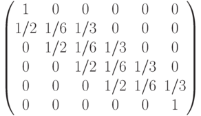
Example 1. Transition matrix specified Find the transition matrix

Solution. Let's use the formula

Multiplying the matrices, we finally get:

§4. Stationary distribution. Limit Probability Theorem

The probability distribution at an arbitrary point in time can be found using the total probability formula

(7)

It may turn out that it does not depend on time. Let's call stationary distribution vector , satisfying the conditions

where are the transition probabilities.

If in a Markov chain then for any

This statement follows by induction from (7) and (8).

Let us present the formulation of the theorem on limiting probabilities for one important class of Markov chains.

Theorem 1. If for some >0 all elements of the matrix are positive, then for any , for

, (9)

Where stationary distribution with a some constant satisfying the inequality 0< h <1.

Since , then according to the conditions of the theorem, from any state you can get to any state in time with a positive probability. The conditions of the theorem exclude chains that are in some sense periodic.

If the conditions of Theorem 1 are met, then the probability that the system is in a certain state in the limit does not depend on the initial distribution. Indeed, from (9) and (7) it follows that for any initial distribution ,

Let us consider several examples of Markov chains for which the conditions of Theorem 1 are not met. It is not difficult to verify that such examples are examples. In the example, the transition probabilities have limits, but these limits depend on the initial state. In particular, when

In other examples, the probability ranges for obviously do not exist.

Let's find the stationary distribution in example 1. We need to find the vector satisfying conditions (8):

;

Hence, Thus, a stationary distribution exists, but not all coordinate vectors are positive.

For the polynomial scheme, random variables were introduced equal to the number of outcomes of a given type. Let us introduce similar quantities for Markov chains. Let be the number of times the system enters the state in time . Then the frequency of the system hitting the state . Using formulas (9), we can prove that when approaches . To do this, you need to obtain asymptotic formulas for and and use Chebyshev’s inequality. Here is the derivation of the formula for . Let's represent it in the form

(10)

where, if, and otherwise. Because

then, using the property of mathematical expectation and formula (9), we obtain

By virtue of Theorem 1, the triple term on the right side of this equality is a partial sum of a convergent series. Putting , we get

Because the

From formula (11), in particular, it follows that

You can also get a formula for which is used to calculate the variance.

§5. Proof of the theorem on limiting probabilities in a Markov chain

Let us first prove two lemmas. Let's put

Lemma 1. There are limits for any

Proof. Using equation (3) with we obtain

Thus, the sequences are both monotonic and limited. This implies the statement of Lemma 1.

Lemma 2. If the conditions of Theorem 2 are met, then there are constants , such that

For any

where , means summation over all for which is positive, and summation over the rest . From here

. (12)

Since under the conditions of Theorem 1 the transition probabilities for all , then for any

And due to the finite number of states

Let us now estimate the difference . Using equation (3) with , , we obtain

From here, using (8)-(10), we find

Combining this relation with inequality (14), we obtain the statement of the lemma.

Go to the proof of the theorem. Since the sequences are monotonic, then

0<. (15)

From this and Lemma 1 we find

Therefore, when you get and

Positivity follows from inequality (15). Passing to the limit at and in equation (3), we obtain that satisfies equation (12). The theorem has been proven.

§6. Applications of Markov chains

Markov chains serve as a good introduction to the theory of random processes, i.e. the theory of simple sequences of a family of random variables, usually depending on a parameter, which in most applications plays the role of time. It is intended primarily to fully describe both long-term and local behavior of a process. Here are some of the most studied issues in this regard.

Brownian motion and its generalizations - diffusion processes and processes with independent increments . The theory of random processes contributed to a deepening of the connection between the theory of probability, the theory of operators and the theory of differential equations, which, among other things, was important for physics and other applications. Applications include processes of interest to actuarial (insurance) mathematics, queuing theory, genetics, traffic control, electrical circuit theory, and inventory theory.

Martingales . These processes preserve enough properties of Markov chains that important ergodic theorems remain valid for them. Martingales differ from Markov chains in that when the current state is known, only the mathematical expectation of the future, but not necessarily the probability distribution itself, does not depend on the past. In addition to the fact that the theory of martingales is an important tool for research, it has enriched the theory of random processes arising in statistics, the theory of nuclear fission, genetics and information theory with new limit theorems.

Stationary processes . The oldest known ergodic theorem, as noted above, can be interpreted as a result describing the limiting behavior of a stationary random process. Such a process has the property that all the probabilistic laws that it satisfies remain invariant with respect to time shifts. The ergodic theorem, first formulated by physicists as a hypothesis, can be represented as a statement that, under certain conditions, the ensemble average coincides with the time average. This means that the same information can be obtained from long-term observation of a system and from simultaneous (and instantaneous) observation of many independent copies of the same system. The law of large numbers is nothing more than a special case of Birkhoff's ergodic theorem. Interpolation and prediction of the behavior of stationary Gaussian processes, understood in a broad sense, serve as an important generalization of classical least squares theory. The theory of stationary processes is a necessary research tool in many fields, for example, in communication theory, which deals with the study and creation of systems that transmit messages in the presence of noise or random interference.

Markov processes (processes without aftereffects) play a huge role in modeling queuing systems (QS), as well as in modeling and choosing a strategy for managing socio-economic processes occurring in society.

Markov chain can also be used to generate texts. Several texts are supplied as input, then a Markov chain is built with the probabilities of one word following another, and the resulting text is created based on this chain. The toy turns out to be very entertaining!

Conclusion

Thus, in our course work we were talking about the Markov chain circuit. We learned in what areas and how it is used, independent tests proved the theorem on limiting probabilities in a Markov chain, gave examples for a typical and homogeneous Markov chain, as well as for finding the transition matrix.

We have seen that the Markov chain design is a direct generalization of the independent test design.

List of used literature

1. Chistyakov V.P. Probability theory course. 6th ed., rev. − St. Petersburg: Lan Publishing House, 2003. − 272 p. − (Textbook for universities. Special literature).

2. Gnedenko B.V. Probability theory course.

3. Gmurman V.E. Theory of Probability and Mathematical Statistics.

4. Ventzel E.S. Probability theory and its engineering applications.

5. Kolmogorov A.N., Zhurbenko I.G., Prokhorov A.V. Introduction to probability theory. − Moscow-Izhevsk: Institute of Computer Research, 2003, 188 pp.

6. Katz M. Probability and related issues in physics.

(Andrei Andreevich Markov (1856-1922) - Russian mathematician, academician)

Definition. A process occurring in a physical system is called Markovsky, if at any moment in time the probability of any state of the system in the future depends only on the state of the system at the current moment and does not depend on how the system came to this state.

Definition. Markov chain called a sequence of trials, in each of which only one of the K incompatible events Ai from the full group. In this case, the conditional probability Pij(S) what's in S-th test the event will come Aj provided that in ( S – 1 ) – the event occurred during the test Ai, does not depend on the results of previous tests.

Independent trials are a special case of a Markov chain. The events are called System states, and tests - Changes in system states.

Based on the nature of changes in states, Markov chains can be divided into two groups.

Definition. Discrete-time Markov chain It is called a circuit whose states change at certain fixed moments in time. Continuous-time Markov chain It is called a circuit whose states can change at any random moments in time.

Definition. Homogeneous It is called a Markov chain if the conditional probability Pij transition of the system from the state I In state J does not depend on the test number. Probability Pij called Transition probability.

Suppose the number of states is finite and equal K.

Then the matrix composed of conditional transition probabilities will look like:

This matrix is called System transition matrix.

Since each row contains the probabilities of events that form a complete group, it is obvious that the sum of the elements of each row of the matrix is equal to one.

Based on the transition matrix of the system, one can construct the so-called System state graph, it is also called Labeled State Graph. This is convenient for a visual representation of the circuit. Let's look at the order of constructing graphs using an example.

Example. Using a given transition matrix, construct a state graph.

Since the matrix is of fourth order, then, accordingly, the system has 4 possible states.

Let Pij(N) – the probability that as a result N tests the system will go from the state I in a state J, R – some intermediate state between states I AND J. Probabilities of transition from one state to another Pij(1) = Pij.

Then the probability Pij(N) can be found using a formula called Markov equality:

Here T– the number of steps (trials) during which the system transitioned from the state I In state R.

In principle, Markov's equality is nothing more than a slightly modified formula for total probability.

Knowing the transition probabilities (i.e. knowing the transition matrix P1), we can find the probabilities of transition from state to state in two steps Pij(2) , i.e. matrix P2, knowing it - find the matrix P3, etc.

Direct application of the formula obtained above is not very convenient, therefore, you can use the techniques of matrix calculus (after all, this formula is essentially nothing more than a formula for multiplying two matrices).

Then in general form we can write:

In general, this fact is usually formulated in the form of a theorem, however, its proof is quite simple, so I will not give it.

Example. Transition matrix specified P1. Find matrix P3.

Definition. Matrices whose sums of elements of all rows are equal to one are called Stochastic. If for some P all matrix elements Rp are not equal to zero, then such a transition matrix is called Regular.

In other words, regular transition matrices define a Markov chain in which each state can be reached through P steps from any state. Such Markov chains are also called Regular.

Theorem. (limit probability theorem) Let a regular Markov chain with n states be given and P be its transition probability matrix. Then there is a limit and a matrix P(¥ ) has the form:

Markov process- a random process occurring in the system, which has the property: for each moment of time t 0, the probability of any state of the system in the future (at t>t 0) depends only on its state in the present (at t = t 0) and does not depend on when and how the system came to this state (i.e. how the process developed in the past).

In practice, we often encounter random processes that, to varying degrees of approximation, can be considered Markovian.

Any Markov process is described using state probabilities and transition probabilities.

Probabilities of states P k (t) of a Markov process are the probabilities that the random process (system) at time t is in state S k:

Transition probabilities of a Markov process are the probabilities of transition of a process (system) from one state to another:

The Markov process is called homogeneous, if the transition probabilities per unit time do not depend on where on the time axis the transition occurs.

The simplest process is Markov chain– Markov random process with discrete time and discrete finite set of states.

When analyzed, the Markov chains are state graph, on which all states of the chain (system) and non-zero probabilities are marked in one step.

A Markov chain can be thought of as if a point representing a system moves randomly through a state graph, dragging from state to state in one step or staying in the same state for several steps.

The transition probabilities of a Markov chain in one step are written in the form of a matrix P=||P ij ||, which is called the transition probability matrix or simply the transition matrix.

Example: the set of states of students of the specialty is as follows:

S 1 – freshman;

S 2 – sophomore…;

S 5 – 5th year student;

S 6 – specialist who graduated from a university;

S 7 – a person who studied at a university, but did not graduate.

From state S 1 within a year, transitions to state S 2 are possible with probability r 1 ; S 1 with probability q 1 and S 7 with probability p 1, and:

r 1 +q 1 +p 1 =1.

Let's build a state graph for this Markov chain and mark it with transition probabilities (non-zero).

Let's create a matrix of transition probabilities:

Transition matrices have the following properties:

All their elements are non-negative;

Their row sums are equal to one.

Matrices with this property are called stochastic.

Transition matrices allow you to calculate the probability of any Markov chain trajectory using the probability multiplication theorem.

For homogeneous Markov chains, transition matrices do not depend on time.

When studying Markov chains, the ones of greatest interest are:

Probabilities of transition in m steps;

Distribution over states at step m→∞;

Average time spent in a certain state;

Average time to return to this state.

Consider a homogeneous Markov chain with n states. To obtain the probability of transition from state S i to state S j in m steps, in accordance with the total probability formula, one should sum the products of the probability of transition from state Si to the intermediate state Sk in l steps by the probability of transition from Sk to Sj in the remaining m-l steps, i.e. .

This relation is for all i=1, …, n; j=1, …,n can be represented as a product of matrices:

P(m)=P(l)*P(m-l).

Thus we have:

P(2)=P(1)*P(1)=P 2

P(3)=P(2)*P(1)=P(1)*P(2)=P 3, etc.

P(m)=P(m-1)*P(1)=P(1)*P(M-1)=P m ,

which makes it possible to find the probabilities of transition between states in any number of steps, knowing the transition matrix in one step, namely P ij (m) - an element of the matrix P(m) is the probability of moving from state S i to state S j in m steps.

Example: The weather in a certain region alternates between rainy and dry over long periods of time. If it rains, then with probability 0.7 it will rain the next day; If the weather is dry on a certain day, then with a probability of 0.6 it will persist the next day. It is known that the weather was rainy on Wednesday. What is the probability that it will be rainy next Friday?

Let's write down all the states of the Markov chain in this problem: D – rainy weather, C – dry weather.

Let's build a state graph:

Answer: p 11 = p (D heel | D avg) = 0.61.

The probability limits р 1 (m), р 2 (m),…, р n (m) for m→∞, if they exist, are called limiting probabilities of states.

The following theorem can be proven: if in a Markov chain you can go from + each state (in a given number of steps) to each other, then the limiting probabilities of the states exist and do not depend on the initial state of the system.

Thus, as m→∞, a certain limiting stationary regime is established in the system, in which each of the states occurs with a certain constant probability.

The vector p, composed of marginal probabilities, must satisfy the relation: p=p*P.

Average time spent in the state S i for time T is equal to p i *T, where p i - marginal probability of state S i . Average time to return to state S i is equal to .

Example.

For many economic problems, it is necessary to know the alternation of years with certain values of annual river flows. Of course, this alternation cannot be determined absolutely precisely. To determine the probabilities of alternation (transition), we divide the flows by introducing four gradations (states of the system): first (lowest flow), second, third, fourth (highest flow). For definiteness, we will assume that the first gradation is never followed by the fourth, and the fourth by the first due to the accumulation of moisture (in the ground, reservoir, etc.). Observations have shown that in a certain region other transitions are possible, and:

a) from the first gradation you can move to each of the middle ones twice as often as again to the first, i.e.

p 11 =0.2; p 12 =0.4; p 13 =0.4; p 14 =0;

b) from the fourth gradation, transitions to the second and third gradations occur four and five times more often than returns as in the second, i.e.

hard, i.e.

in the fourth, i.e.

p 41 =0; p 42 =0.4; p 43 =0.5; p 44 =0.1;

c) from the second to other gradations can only be less frequent: in the first - two times less, in the third by 25%, in the fourth - four times less often than the transition to the second, i.e.

p 21 =0.2;p 22 =0.4; p 23 =0.3; p 24 =0.1;

d) from the third gradation, a transition to the second gradation is as likely as a return to the third gradation, and transitions to the first and fourth gradations are four times less likely, i.e.

p 31 =0.1; p 32 =0.4; p 33 =0.4; p 34 =0.1;

Let's build a graph:

Let's create a matrix of transition probabilities:

Let's find the average time between droughts and high-water years. To do this, you need to find the limit distribution. It exists because the condition of the theorem is satisfied (the matrix P2 does not contain zero elements, i.e., in two steps you can go from any state of the system to any other).

Where p 4 =0.08; p 3 =; p 2 =; p 1 =0.15

The frequency of return to state S i is equal to .

Consequently, the frequency of dry years is on average 6.85, i.e. 6-7 years, and rainy years 12.