Design of experiments. History of experimental planning o Ex post facto plans
A psychological experiment begins with instructions, or more precisely, with the establishment of certain relationships between the subject and the experimenter. Another task that the researcher faces is sampling: with whom the experiment should be conducted so that its results can be considered reliable. The end of the experiment is processing its results, interpreting the data obtained and presenting them to the psychological community.
|
Procedures |
|
|
preparatory |
1. the need to solve a certain problem, its awareness, study, selection of literature. 2.formulation of tasks 3.definition of the object and subject of research 4.formulation of the hypothesis 5. selection of methods and techniques. |
|
research |
Collect evidence using different methods. Various steps in a series of studies are carried out. |
|
Processing of research data |
Quantitative and qualitative analysis of the study. 1.analysis of the recorded factor. 2. establishing a connection: a recorded fact - a hypothesis. 3. identification of recurring factors. Statistical processing, drawing up tables, graphs, etc. takes place. |
|
Data interpretation. Conclusion |
1. establishing the correctness or fallacy of the research hypothesis. 2. correlation of results with existing concepts and theories. |
The concept of control is used in science in two, somewhat interrelated, different senses.
The second meaning given to the word control refers to the exclusion of the effects of variables chosen by the researcher in experiments or observations conducted under artificially created conditions - i.e. their influence is “controlled”. Eliminating variation in controlled variables makes it possible to more effectively assess the influence of another variable, called. independent, on the measured, or dependent, variable. Such exclusion of extraneous sources of variation allows the researcher to reduce the uncertainty accompanying natural conditions, which obscures the picture of cause-and-effect relationships, etc. get more accurate facts.
The variable can be controlled in two ways. ways. The simplest method is to hold the controlled variable constant across all conditions or groups of subjects; an example would be eliminating gender variation by using only men or only women as subjects. With the second method, a certain influence of the controlled variable is allowed, but an attempt is made to keep it at the same level under all conditions or in all groups of subjects; resp. An example is the involvement of an equal number of men and women in each of the groups taking part in the experiment.
Controlling critical variables is not always easy or even possible. An example here would be astronomy. Of course, it is not possible to manipulate the movement of stars and planets or other celestial bodies, which would make it possible to put observations under complete control. However, it is possible to plan observations in advance in order to take into account the occurrence of certain natural events in advance - the so-called. natural experiments - and thereby achieve a certain degree of control in observations.
Experiment planning
Tutorial
Voronezh 2013
FGBOUVPO "Voronezh State Technical University"
Experiment planning
Approved by the University Editorial and Publishing Council as a teaching aid
Voronezh 2013
UDC: 629.7.02
Popov experiment: textbook. allowance. Voronezh: FGBOUVPO "Voronezh State Technical University", 20p.
The tutorial discusses the issue of planning an experiment. The publication meets the requirements of the State educational standard higher professional education in the direction 652100 “Aircraft Engineering”, specialty 160201 “Aircraft and Helicopter Engineering”, discipline “Planning of Experiments and Processing of Results”.
The textbook was developed within the framework of the implementation of the federal target program “Scientific and scientific-pedagogical personnel of innovative Russia” for 2009 – 2013, agreement No. 14.B37.21.1824, related to the implementation of research work (project) on the topic “Research, design development continuous elliptical fairings of air intakes of aircraft engines and modeling of the technological process"
Table 3. Il. 8. Bibliography: 4 titles.
Scientific editor Ph.D. tech. Sciences, Associate Professor
Reviewers: Irkut branch in Voronezh (deputy director, candidate of technical sciences, senior researcher);
Cand. tech. sciences
© Design. FGBOUVPO "Voronezh State Technical University", 2013
Introduction
Traditional research methods involve experiments that require a lot of effort, effort and resources.
Experiments, as a rule, are multifactorial and are associated with optimizing the quality of materials, finding optimal conditions for carrying out technological processes, developing the most rational equipment designs, etc. The systems that serve as the object of such research are very often so complex that they cannot be studied theoretically within a reasonable time. Therefore, despite the significant amount of research work performed, due to the lack of a real opportunity to sufficiently study a significant number of research objects, as a result, many decisions are made on the basis of random information and are therefore far from optimal.
Based on the above, there is a need to find a way that allows research work to be carried out at an accelerated pace and ensures the adoption of decisions that are close to optimal. This was the path to statistical methods for planning experiments, proposed by the English statistician Ronald Fisher (late twenties). He was the first to show the advisability of simultaneous variation of all factors, as opposed to the widespread one-factor experiment.
The use of experimental planning makes the experimenter's behavior purposeful and organized, significantly contributing to increased productivity and the reliability of the results obtained. An important advantage is its versatility and suitability in the vast majority of areas of research. In our country, experimental planning has been developing since 1960 under the leadership of. However, even a simple planning procedure is very difficult, which is due to a number of reasons, such as incorrect application of planning methods, choice of a less than optimal research path, lack of practical experience, insufficient mathematical preparedness of the experimenter, etc.
The purpose of this textbook is to familiarize students with the most commonly used and simple methods of experiment planning and to develop practical application skills. The problem of process optimization is considered in more detail.
1 Basic concepts of experimental design
Planning an experiment has its own specific terminology. Let's look at some general terms.
An experiment is a system of operations, influences and (or) observations aimed at obtaining information about an object during research tests.
Experience is the reproduction of the phenomenon under study under certain experimental conditions with the possibility of recording its results. Experience is a separate elementary part of the experiment.
Experimental planning is the procedure for selecting the number of experiments and the conditions for conducting them necessary to solve a given problem with the required accuracy. All factors that determine the process are changed simultaneously according to special rules, and the results of the experiment are presented in the form of a mathematical model.
The problems for which experimental design can be used are extremely diverse. These include: the search for optimal conditions, the construction of interpolation formulas, the selection of essential factors, the assessment and refinement of constants of theoretical models, the selection of the most acceptable from a certain set of hypotheses about the mechanism of phenomena, the study of composition-property diagrams, etc.
Finding optimal conditions is one of the most common scientific and technical problems. They arise at the moment when the possibility of carrying out the process has been established and it is necessary to find the best (optimal) conditions for its implementation. Such problems are called optimization problems. The process of solving them is called the optimization process or simply optimization. Examples of optimization problems are choosing the optimal composition of multicomponent mixtures and alloys, increasing the productivity of existing installations, improving product quality, reducing the cost of obtaining it, etc.
The following stages are identified in constructing a mathematical model:
1. collection and analysis of a priori information;
2. selection of factors and output variables, areas of experimentation;
3. selection of a mathematical model with the help of which experimental data will be presented;
5. determination of the data analysis method;
6. conducting an experiment;
7. checking the statistical premises for the obtained experimental data;
8. processing of results;
Factors determine the state of an object. The main requirement for factors is controllability. Controllability means establishing the desired factor value (level) and maintaining it throughout the experiment. This is the peculiarity of an active experiment. Factors can be quantitative or qualitative. Examples of quantitative factors are temperature, pressure, concentration, etc. Their levels correspond to a numerical scale. Various catalysts, apparatus designs, treatment methods, teaching methods are examples of qualitative factors. The levels of such factors do not correspond to a numerical scale, and their order does not matter.
Output variables are reactions (responses) to the influence of factors. The response depends on the specifics of the study and can be economic (profit, profitability), technological (output, reliability), psychological, statistical, etc. The optimization parameter must be effective in terms of achieving the goal, universal, quantitative, expressible as a number, having a physical meaning, to be simple and easy to calculate.
Computer time costs can be significantly reduced if an experimental factorial mathematical model is used at the parameter optimization stage. Experimental factor models, unlike theoretical ones, do not use physical laws that describe the processes occurring in objects, but represent some formal dependencies of output parameters on the internal and external parameters of design objects.
An experimental factor model can be built on the basis of conducting experiments directly on the technical object itself (physical experiments), or computational experiments on a computer with a theoretical model.
Picture 1
When constructing an experimental factor model, the modeling object (the designed technical system) is presented in the form of a “black box”, the input of which is supplied by some variables X and Z, and at the output the variables Y can be observed and recorded.
During the experiment, changes in variables X and Z lead to changes in output variables Y. To build a factor model, it is necessary to record these changes and carry out the necessary statistical processing to determine the parameters of the model.
When conducting a physical experiment, the variables X can be controlled by changing their value according to a given law. Z variables are uncontrollable and take random values. In this case, the values of the variables X and Z can be monitored and recorded using appropriate measuring instruments. In addition, the object is affected by some variables E that cannot be observed and controlled. Variables X= (x1, x2,..., xn) are called controlled; variables Z = (z1, z2,…… zm) are controlled but uncontrollable, and variables E = (ε1, ε2,..., εl) are uncontrollable and uncontrollable.
The variables X and Z are called factors. Factors X are controllable and change as deterministic variables, and factors Z are uncontrollable, changing randomly over time, i.e. Z are random processes. The space of controlled variables - factors X and Z - forms a factor space.
The output variable Y is a vector of dependent variables of the modeled object. It is called the response, and the dependence of Y on factors X and Z is the response function. The geometric representation of a response function is called a response surface.
Variable E acts uncontrollably during the experiment. If we assume that factors X and Z are stabilized in time and maintain constant values, then under the influence of variables E the response function Y can change both systematically and randomly. In the first case, we talk about systematic interference, and in the second, about random interference. It is believed that random noise has probabilistic properties that do not change over time.
The occurrence of interference is caused by errors in the methods of conducting physical experiments, errors in measuring instruments, uncontrolled changes in the parameters and characteristics of the object and the external environment.
In computational experiments, the object of study is a theoretical mathematical model, on the basis of which it is necessary to obtain an experimental factor model. To obtain it, it is necessary to determine the structure and numerical values of the model parameters.
The structure of the model is understood as the type of mathematical relationships between factors X, Z and response Y. The parameters are the coefficients of the factor model equations. The structure of the model is usually chosen based on a priori information about the object, taking into account the purpose and subsequent use of the model. The task of determining model parameters is completely formalized. It is solved using regression analysis methods. Experimental factor models are also called regression models.
The regression model can be represented by the expression
![]() (1.1)
(1.1)
where B is the vector of parameters of the factor model.
The form of the vector function φ is determined by the chosen structure of the model and is considered given, and parameters B are subject to determination based on the experimental results.
There are passive and active experiments.
An experiment is called passive when the values of the factors cannot be controlled and they take random values. In such an experiment, only factors Z exist. During the experiment, at certain points in time, the values of factors Z and response functions Y are measured. After N experiments, the information obtained is processed by statistical methods that make it possible to determine the parameters of the factor model. This approach to constructing a mathematical model underlies the statistical testing method (Monte Carlo).
An experiment is called active when the values of factors are set and maintained unchanged at specified levels in each experiment in accordance with the experimental plan. Therefore, in this case there are only controllable factors X.
The main features of experimental factor models are the following: they are statistical; represent relatively simple functional dependencies between estimates of mathematical expectations of the output parameters of an object from its internal and external parameters; provide an adequate description of the established dependencies only in the region of the factor space in which the experiment is implemented. Statistically, a regression model describes the behavior of an object on average, characterizing its non-random properties, which are fully manifested only when experiments are repeated many times under constant conditions.
2 Basic principles of experimental design
To obtain an adequate mathematical model, it is necessary to ensure that certain experimental conditions are met. A model is called adequate if, in a specified area of variation of factors X, the values of response functions Y obtained using the model differ from the true ones by no more than a given value. Methods for constructing experimental factor models are considered in the theory of experimental design.
The purpose of planning an experiment is to obtain maximum information about the properties of the object under study with a minimum of experiments. This approach is due to the high cost of experiments, both physical and computational, and at the same time the need to build an adequate model.
When planning active experiments, the following principles are used:
– refusal to completely enumerate all possible states of an object;
– gradual complication of the structure of the mathematical model;
– comparison of the experimental results with the magnitude of random noise;
– randomization of experiments;
A detailed understanding of the properties of the response surface can be obtained only by using a dense discrete grid of factor values covering the entire factor space. At the nodes of this multidimensional grid there are plan points at which experiments are carried out. The choice of factor model structure is based on postulating a certain degree of smoothness of the response surface. Therefore, in order to reduce the number of experiments, a small number of plan points are taken for which the experiment is carried out.
With a large level of random noise, a large scatter of response function values Y is obtained in experiments conducted at the same point in the plan. In this case, it turns out that the higher the noise level, the more likely the simple model is to work. The lower the level of interference, the more accurate the factor model should be.
In addition to random interference, systematic interference may occur during the experiment. The presence of this interference is practically undetectable and the result of its impact on the function cannot be controlled. However, if, through the appropriate organization of experiments, a random situation is artificially created, then the systematic interference can be transferred to the category of random. This principle of organizing an experiment is called randomization of systematically acting interference.
The presence of interference leads to experimental errors. Errors are divided into systematic and random, according to the names of the factors causing them - interference.
Randomization of experiments is carried out only in physical experiments. It should be noted that in these experiments, a systematic error can also be generated, along with the previously noted factors, by inaccurate setting of the values of controlled factors, due to poor calibration of the instruments for measuring them (instrumental error), design or technological factors.
Factors in an active experiment are subject to certain requirements. They should be:
– controlled (setting specified values and maintaining them constant during the experiment);
– joint (their mutual influence should not disrupt the functioning of the object);
– independent (the level of any factor must be set independently of the levels of the others);
– unambiguous (some factors should not be a function of others);
– directly affecting the output parameters.
The choice of optimization parameters (optimization criteria) is one of the main stages of work at the stage of preliminary study of the research object, since the correct formulation of the problem depends on the correct choice of the optimization parameter, which is a function of the goal.
An optimization parameter is understood as a characteristic of a goal, specified quantitatively. The optimization parameter is a reaction (response) to the influence of factors that determine the behavior of the selected system.
Real objects or processes are usually very complex. They often require simultaneous consideration of several, sometimes very many, parameters. Each object can be characterized by the entire set of parameters, or any subset of this set, or by one single optimization parameter. In the latter case, other process characteristics no longer act as optimization parameters, but serve as restrictions. Another way is to construct a generalized optimization parameter as a function of a set of initial ones.
An optimization parameter (Response Function) is a feature by which the process is optimized. It must be quantitative, given by number. The set of values that an optimization parameter can take is called its domain of definition. Areas of definition can be continuous and discrete, limited and unlimited. For example, the output of a reaction is an optimization parameter with a continuous limited domain. It can vary from 0 to 100%. The number of defective products, the number of grains on a thin section of an alloy, the number of blood cells in a blood sample - these are examples of parameters with a discrete definition range limited from below.
Quantitative assessment of the optimization parameter is not always possible in practice. In such cases, a technique called ranking is used. In this case, the optimization parameters are assigned ratings - ranks on a pre-selected scale: two-point, five-point, etc. The rank parameter has a discrete limited definition area. In the simplest case, the area contains two values (yes, no; good, bad). This may correspond, for example, to good products and defective products.
2.1 Types of optimization parameters
Depending on the object and goal, optimization parameters can be very diverse. Let's introduce some classification. Real situations are usually quite complex. They often require several, sometimes very many, parameters. In principle, each object can be characterized by the entire set of parameters shown in Figure 2, or any subset of this set. Movement towards the optimum is possible if a single optimization parameter is selected. Then other characteristics of the process no longer act as optimization parameters, but serve as restrictions. Another way is to construct a generalized optimization parameter as a function of a set of initial ones.

Let us comment on some elements of the scheme.
Economic optimization parameters, such as profit, cost and profitability, are usually used when studying existing industrial facilities, while it makes sense to evaluate the costs of an experiment in any research, including laboratory ones. If the price of the experiments is the same, the costs of the experiment are proportional to the number of experiments that need to be carried out to solve a given problem. This largely determines the choice of experimental design.
Among the technical and economic parameters, productivity is the most widespread. Parameters such as durability, reliability and stability are associated with long-term observations. There is some experience of using them in the study of expensive, critical objects, such as electronic equipment.
Almost all studies have to take into account the quantity and quality of the resulting product. Yield is used as a measure of the amount of product, for example, the percentage of yield of a chemical reaction, the yield of suitable products.
Quality indicators are extremely varied. In the diagram they are grouped by property type. The characteristics of the quantity and quality of the product form a group of technical and technological parameters.
Under the heading “other” are grouped various parameters that are less common, but no less important. This includes statistical parameters used to improve the characteristics of random variables or random functions. As examples, we will name problems of minimizing the dispersion of a random variable, reducing the number of emissions of a random process beyond a fixed level, etc. The last problem arises, in particular, when choosing the optimal settings of automatic regulators or when improving the properties of threads (wire, yarn, artificial fiber and etc.).
2.2 Requirements for optimization parameters
1) the optimization parameter must be quantitative.
2) the optimization parameter must be expressed as a single number. Sometimes it comes naturally, like recording a reading from a device. For example, the speed of a car is determined by the number on the speedometer. Often you have to do some calculations. This happens when calculating the yield of a reaction. In chemistry, it is often necessary to obtain a product with a given ratio of components, for example, A:B = 3:2. One of the possible solutions to such problems is to express the ratio with a single number (1.5) and use the value of deviations (or squares of deviations) from this number as an optimization parameter.
3) uniqueness in a statistical sense. A given set of factor values must correspond to one optimization parameter value, while the converse is not true: different sets of factor values can correspond to the same parameter value.
4) the most important requirement for optimization parameters is its ability to truly effectively evaluate the functioning of the system. The idea of an object does not remain constant during the course of the study. It changes as information accumulates and depending on the results achieved. This leads to a consistent approach when choosing an optimization parameter. For example, in the first stages of process research, product yield is often used as an optimization parameter. However, in the future, when the possibility of increasing the yield has been exhausted, they begin to be interested in such parameters as cost, product purity, etc. Assessing the effectiveness of the system can be carried out both for the entire system as a whole, and by assessing the effectiveness of a number of subsystems that make up this system. But at the same time, it is necessary to take into account the possibility that the optimality of each of the subsystems in terms of its optimization parameter “does not exclude the possibility of the death of the system as a whole.” This means that an attempt to achieve an optimum taking into account some local or intermediate optimization parameter may be ineffective or even lead to failure.
5) requirement of universality or completeness. The universality of an optimization parameter is understood as its ability to comprehensively characterize an object. In particular, technological parameters are not universal enough: they do not take into account economics. For example, generalized optimization parameters, which are constructed as functions of several particular parameters, are universal.
6) the optimization parameter should preferably have a physical meaning, be simple and easy to calculate. The requirement for physical meaning is associated with the subsequent interpretation of the experimental results. It is not difficult to explain what maximum extraction means, maximum content of a valuable component. These and similar technological optimization parameters have a clear physical meaning, but sometimes they may not meet, for example, the requirement of statistical efficiency. Then it is recommended to proceed to transforming the optimization parameter. The second requirement, i.e. simplicity and ease of computability, are also very important. For separation processes, thermodynamic optimization parameters are more universal. However, in practice they are rarely used: their calculation is quite difficult. Of the above two requirements, the first is more significant, because it is often possible to find the ideal characteristics of the system and compare it with the actual characteristics.
2.3Factors
After choosing the object of study and the optimization parameter, you need to consider all the factors that may influence the process. If any significant factor turns out to be unaccounted for and takes arbitrary values not controlled by the experimenter, this will significantly increase the experimental error. By maintaining this factor at a certain level, a false idea of the optimum may be obtained, since there is no guarantee that the resulting level is optimal.
On the other hand, a large number of factors increases the number of experiments and the dimension of the factor space.
The choice of experimental factors is very important; the success of optimization depends on it.
A factor is a measured variable that takes on a certain value at some point in time and influences the object of study.
Factors must have a domain of definition within which its specific values are specified. The domain of definition can be continuous or discrete. When planning an experiment, the values of the factors are taken to be discrete, which is associated with the levels of the factors. In practical problems, the area of determining factors has limitations that are either fundamental or technical in nature.
Factors are divided into quantitative and qualitative.
Quantitative factors include those factors that can be measured, weighed, etc.
Qualitative factors are various substances, technological methods, devices, performers, etc.
Although a numerical scale does not correspond to qualitative factors, when planning an experiment, a conditional ordinal scale is applied to them in accordance with the levels, i.e. coding is performed. The order of levels here is arbitrary, but after coding it is fixed.
2.3.1 Requirements for experimental factors
1) Factors must be controllable, this means that the selected desired value of the factor can be maintained constant throughout the experiment. An experiment can only be planned if the levels of factors are subject to the will of the experimenter. For example, the experimental setup is installed in an open area. Here we cannot control the air temperature, it can only be monitored, and therefore, when performing experiments, we cannot take temperature into account as a factor.
2) To accurately determine a factor, you need to indicate the sequence of actions (operations) with the help of which its specific values are established. This definition is called operational. Thus, if the factor is the pressure in some apparatus, then it is absolutely necessary to indicate at what point and with what instrument it is measured and how it is set. The introduction of an operational definition provides an unambiguous understanding of the factor.
3) The accuracy of factor measurements should be as high as possible. The degree of accuracy is determined by the range of changes in factors. In long processes, measured over many hours, minutes can be ignored, but in fast processes, fractions of a second must be taken into account.
The study becomes significantly more complicated if the factor is measured with a large error or the values of the factors are difficult to maintain at the selected level (the level of the factor “floats”), then special research methods have to be used, for example, confluence analysis.
4) Factors must be unambiguous. It is difficult to control a factor that is a function of other factors. But other factors may participate in planning, such as relationships between components, their logarithms, etc. The need to introduce complex factors arises when there is a desire to represent the dynamic features of an object in static form. For example, it is necessary to find the optimal mode for raising the temperature in the reactor. If it is known with respect to temperature that it should increase linearly, then instead of a function (in this case linear), the tangent of the angle of inclination, i.e., the gradient, can be used as a factor.
5) When planning an experiment, several factors are simultaneously changed, so it is necessary to know the requirements for a set of factors. First of all, the requirement of compatibility is put forward. The compatibility of factors means that all their combinations are feasible and safe. Incompatibility of factors is observed at the boundaries of the areas of their definition. You can get rid of it by reducing the areas. The situation becomes more complicated if incompatibility occurs within the domains of definition. One possible solution is to split it into subdomains and solve two separate problems.
6) When planning an experiment, the independence of factors is important, i.e. the possibility of establishing a factor at any level, regardless of the levels of other factors. If this condition is not met, then it is impossible to plan the experiment.
2.3.2 Requirements for a combination of factors
When designing an experiment, several factors are usually changed simultaneously. Therefore, it is very important to formulate the requirements that apply to a combination of factors. First of all, the requirement of compatibility is put forward. The compatibility of factors means that all their combinations are feasible and safe. This is a very important requirement. Imagine that you acted carelessly, did not pay attention to the requirement of compatibility of factors and planned such experimental conditions that could lead to an explosion of the installation or tarring of the product. Agree that such a result is very far from optimization goals.
Incompatibility of factors can be observed at the boundaries of the areas of their definition. You can get rid of it by reducing the areas. The situation becomes more complicated if incompatibility occurs within the domains of definition. One possible solution is to split it into subdomains and solve two separate problems.
When planning an experiment, the independence of factors is important, i.e. the ability to establish a factor at any level, regardless of the levels of other factors. If this condition is not met, then it is impossible to plan the experiment. So, we come to the second requirement - the absence of correlation between factors. The requirement of uncorrelation does not mean that there is no connection between the values of the factors. It is enough that the relationship is not linear.
3 Design of the experiment
3.1 Experimental design
When conducting an active experiment, a specific plan for varying factors is set, i.e. the experiment is planned in advance
Experimental plan is a set of data that determines the number, conditions and order of implementation of experiments.
Experimental planning - choosing an experimental plan that meets specified requirements.
A plan point is an ordered set of numerical values of factors corresponding to the conditions of the experiment, i.e., the point in the factor space in which the experiment is carried out. The plan point with number i corresponds to the row vector (3.1):
![]() (3.1)
(3.1)
The total set of such vectors Xi, i= 1, L forms the experimental plan, and the set of different vectors, the number of which we denote by N, is the spectrum of the plan.
In an active experiment, factors can only take fixed values. The fixed value of a factor is called the factor level. The number of factor levels accepted depends on the chosen structure of the factor model and the adopted experimental design. The minimum Xjmin and maximum Xmax, j=l, n (n is the number of factors) levels of all factors highlight in the factor space a certain hyperparallelepiped, which represents the planning area. The planning area contains all possible values of the factors used in the experiment.
Vector ![]() specifies the center point of the planning area. The coordinates of this point Xj0 are usually chosen from relation (3.2)
specifies the center point of the planning area. The coordinates of this point Xj0 are usually chosen from relation (3.2)
![]() (3.2)
(3.2)
Point X0 is called the center of the experiment. It determines the basic level of factors Xj0, j = 1,n. They try to choose the center of the experiment as close as possible to the point that corresponds to the desired optimal values of the factors. For this, a priori information about the object is used.
The interval (or step) of variation of the factor Xj is the value calculated using formulas (3.3, 3.4):
![]() (3.3)
(3.3)
Factors are normalized and their levels are coded. In coded form, the upper level is denoted by +1, the lower -1, and the main level by 0. Factors are normalized based on the ratio (3.5, 3.6):
xj =(Xj-X0j)/ΔXj, (3.5)

Figure 3 – Geometric representation of the planning area with two factors: X1 and X2
Points 1,2,3,4 are the points of the experiment plan. For example, the values of factors X1 and X2 at point 1 are equal to X1min and X2min, respectively, and their normalized values are xlmin = -1, x2min = -1.
After establishing the zero point, factor variation intervals are selected. This is due to the determination of such factor values that in coded values correspond to +1 and –1. Variation intervals are chosen taking into account the fact that the factor values corresponding to levels +1 and –1 must be sufficiently distinguishable from the value corresponding to the zero level. Therefore, in all cases, the value of the variation interval must be greater than twice the squared error of fixing a given factor. On the other hand, an excessive increase in the value of variation intervals is undesirable, since this can lead to a decrease in the efficiency of searching for the optimum. And a very small variation interval reduces the scope of the experiment, which slows down the search for the optimum.
When choosing a variation interval, it is advisable to take into account, if possible, the number of levels of variation of factors in the experimental area. The volume of the experiment and the efficiency of optimization depend on the number of levels.
It is convenient to present the experimental plan in matrix form.
The plan matrix is a rectangular table containing information about the number and conditions of experiments. The rows of the design matrix correspond to experiments, and the columns correspond to factors. The dimension of the design matrix is L x n, where L is the number of experiments, n is the number of factors. When conducting repeated (duplicate) experiments at the same points of the plan, the plan matrix contains a number of matching rows.
1 Designs for one independent variable
The design of a “true” experimental study differs from others in the following important ways:
1) using one of the strategies for creating equivalent groups, most often randomization;
2) the presence of an experimental and at least one control group;
3) completion of the experiment by testing and comparing the behavior of the group that received the experimental intervention (X1) with the group that did not receive the intervention X0.
The classic version of the plan is the plan for 2 independent groups. In psychology, experimental planning began to be used in the first decades of the 20th century.
There are three main versions of this plan. When describing them, we will use the symbolization proposed by Campbell.
Table 5.1
Here R is randomization, X is exposure, O1 is testing the first group, O2 is testing the second group.
1) Two randomized group design with post-exposure testing. Its author is the famous biologist and statistician R. A. Fisher. The structure of the plan is shown in table. 5.1.
Equality between the experimental and control groups is an absolutely necessary condition for the application of this design. Most often, to achieve group equivalence, the randomization procedure is used (see Chapter 4). This plan is recommended for use when it is not possible or necessary to conduct preliminary testing of subjects. If the randomization is done well, then this design is the best and allows you to control most sources of artifacts; in addition, various variants of variance analysis are applicable to it.
After randomization or another procedure for equalizing groups, an experimental intervention is carried out. In the simplest version, only two gradations of the independent variable are used: there is an impact, there is no impact.
If it is necessary to use more than 1 level of exposure, then plans with several experimental groups (according to the number of exposure levels) and one control group are used.
If it is necessary to control the influence of one of the additional variables, then a design with 2 control groups and 1 experimental group is used. Measuring behavior provides material for comparing the 2 groups. Data processing is reduced to the use of traditional estimates for mathematical statistics. Let's consider the case when the measurement is carried out using an interval scale. Student's t-test is used to assess differences in group means. Differences in the variation of the measured parameter between the experimental and control groups are assessed using the F criterion. The corresponding procedures are discussed in detail in textbooks on mathematical statistics for psychologists.
Using a 2 randomized group design with post-exposure testing allows for major sources of internal validity (as defined by Campbell) to be controlled. Since there is no preliminary testing, the interaction effect of the testing procedure and the content of the experimental intervention and the testing effect itself are excluded. The plan allows you to control the influence of group composition, spontaneous dropout, the influence of background and natural development, the interaction of group composition with other factors, and also allows you to eliminate the regression effect due to randomization and comparison of data from the experimental and control groups. However, when conducting most pedagogical and social-psychological experiments, it is necessary to strictly control the initial level of the dependent variable, be it intelligence, anxiety, knowledge or the status of an individual in a group. Randomization is the best possible procedure, but it does not provide an absolute guarantee of the correct choice. When there is doubt about the results of randomization, a pretest design is used.
Table 5.2
2) Design for two randomized groups with pretest and posttest. Let's consider the structure of this plan (Table 5.2).
The pretest design is popular among psychologists. Biologists have more confidence in the randomization procedure. The psychologist knows very well that each person is unique and different from others, and subconsciously strives to capture these differences with the help of tests, not trusting the mechanical randomization procedure. However, the hypothesis of most psychological research, especially in the field of developmental psychology (“formative experiment”), contains a prediction of a certain change in an individual’s property under the influence of an external factor. Therefore, test-exposure-retest designs using randomization and a control group are very common.
In the absence of a group matching procedure, this design becomes a quasi-experimental design (discussed in Section 5.2).
The main source of artifacts that undermines the external validity of a procedure is the interaction of testing with experimental effects. For example, testing the level of knowledge on a certain subject before conducting an experiment on memorizing material can lead to the updating of initial knowledge and to a general increase in memorization productivity. This is achieved by updating mnemonic abilities and creating a memorization mindset.
However, with the help of this plan, other external variables can be controlled. The factor of “history” (“background”) is controlled, since in the interval between the first and second testing both groups are exposed to the same (“background”) influences. However, Campbell notes the need to control for “within-group events,” as well as the effect of non-simultaneous testing in both groups. In reality, it is impossible to ensure that the test and retest are carried out simultaneously in them. The design becomes quasi-experimental, for example:
Typically, non-simultaneous testing is controlled by two experimenters testing two groups simultaneously. The optimal procedure is to randomize the order of testing: testing members of the experimental and control groups is carried out in random order. The same is done with the presentation or non-presentation of experimental influence. Of course, such a procedure requires a significant number of subjects in the experimental and control samples (at least 30-35 people in each).
Natural history and testing effects are controlled by ensuring that they occur equally in the experimental and control groups, and group composition and regression effects [Campbell, 1980] are controlled by the randomization procedure.
The results of applying the test-exposure-retest plan are presented in the table.
When processing data, parametric tests t and F (for data on an interval scale) are usually used. Three t values are calculated: comparison 1) O1 and O2; 2) O3 and O4; 3) O2 and O4. The hypothesis about the significant influence of the independent variable on the dependent variable can be accepted if two conditions are met: a) the differences between O1 and O2 are significant, and between O3 and O4 are insignificant, and b) the differences between O2 and O4 are significant. It is much more convenient to compare not absolute values, but the magnitude of the increase in indicators from the first test to the second (δ(i)). δ(i12) and δ(i34) are calculated and compared using Student's t-test. If the differences are significant, the experimental hypothesis about the influence of the independent variable on the dependent variable is accepted (Table 5.3).
It is also recommended to use Fisher analysis of covariance. In this case, the pre-test indicators are taken as an additional variable, and the subjects are divided into subgroups depending on the pre-test indicators. This results in the following table for data processing using the MANOVA method (Table 5.4).
The use of a “test-exposure-retest” design allows you to control the influence of “side” variables that violate the internal validity of the experiment.
External validity refers to the transferability of data to a real-life situation. The main point that distinguishes the experimental situation from the real one is the introduction of preliminary testing. As we have already noted, the “test-exposure-retest” design does not allow us to control the effect of the interaction of testing and experimental influence: the previously tested subject “sensitizes” - becomes more sensitive to the influence, since in the experiment we measure exactly the dependent variable that we are going to measure influence by varying the independent variable.
Table 5.5
To control external validity, R.L. Solomon’s plan, which he proposed in 1949, is used.
3) The Solomon plan is used when conducting an experiment on four groups:
1. Experiment 1: R O1 X O2
2. Control 1: R O3 O4
3. Experiment 2: R X O5
4. Control 2: R O6
The design includes a study of two experimental and two control groups and is essentially multi-group (2 x 2 type), but for ease of presentation it is discussed in this section.
Solomon's design is a combination of two previously discussed designs: the first, when no pretesting is carried out, and the second, test-exposure-retest. By using the "first part" of the design, the interaction effect of the first test and the experimental treatment can be controlled. Solomon, using his plan, reveals the effect of experimental exposure in four different ways: by comparing 1) O2 - O1; 2) O2 - O4; 3) O5 - O6 and 4) O5 - O3.
If we compare O6 with O1 and O3, we can identify the joint influence of the effects of natural development and “history” (background influences) on the dependent variable.
Campbell, criticizing the data processing schemes proposed by Solomon, suggests not paying attention to preliminary testing and reducing the data to a 2 x 2 scheme, suitable for applying variance analysis (Table 5.5).
Comparison of column averages makes it possible to identify the effect of experimental influence - the influence of the independent variable on the dependent one. Row means show the pretest effect. Comparison of cell means characterizes the interaction of the testing effect and the experimental effect, which indicates the extent of the violation of external validity.
In the case where the effects of preliminary testing and interaction can be neglected, proceed to the comparison of O4 and O2 using the method of covariance analysis. As an additional variable, data from preliminary testing is taken according to the scheme given for the “test-exposure-retest” plan.
Finally, in some cases it is necessary to check the persistence of the effect of the independent variable on the dependent variable over time: for example, to find out whether a new teaching method leads to long-term memorization of the material. For these purposes, the following plan is used:
1 Experiment 1 R O1 X O2
2 Control 1 R O3 O4
3 Experiment 2 R O5 X O6
4 Control 2 R O7 O8
2. Designs for one independent variable and several groups
Sometimes comparing two groups is not enough to confirm or refute an experimental hypothesis. This problem arises in two cases: a) when it is necessary to control external variables; b) if it is necessary to identify quantitative relationships between two variables.
To control external variables, various versions of the factorial experimental design are used. As for identifying a quantitative relationship between two variables, the need to establish it arises when testing an “exact” experimental hypothesis. In an experiment involving two groups, at best, it is possible to establish the fact of a causal relationship between the independent and dependent variables. But between two points you can draw an infinite number of curves. To ensure that there is a linear relationship between two variables, you must have at least three points corresponding to the three levels of the independent variable. Therefore, the experimenter must select several randomized groups and place them in different experimental conditions. The simplest option is a design for three groups and three levels of the independent variable:
Experiment 1: R X1 O1
Experiment 2: R X2 O2
Control: R O3
The control group in this case is the third experimental group, for which the level of the variable X = 0.
In this design, each group is presented with only one level of the independent variable. It is also possible to increase the number of experimental groups according to the number of levels of the independent variable. To process the data obtained using such a plan, the same statistical methods are used as listed above.
Simple “system experimental designs” are, surprisingly, very rarely used in modern experimental research. Maybe researchers are “embarrassed” to put forward simple hypotheses, remembering the “complexity and multidimensionality” of mental reality? The tendency to use designs with many independent variables, indeed to conduct multivariate experiments, does not necessarily contribute to a better explanation of the causes of human behavior. As you know, “a smart person amazes with the depth of his idea, and a fool with the scope of his construction.” It is better to prefer a simple explanation to any complex one, although regression equations where everything equals everything and intricate correlation graphs may impress some dissertation committees.
3 Factorial designs
Factorial experiments are used when it is necessary to test complex hypotheses about the relationships between variables. The general form of such a hypothesis is: “If A1, A2,..., An, then B.” Such hypotheses are called complex, combined, etc. In this case, there can be various relationships between independent variables: conjunction, disjunction, linear independence, additive or multiplicative, etc. Factorial experiments are a special case of multivariate research, during which they try to establish relationships between several independent and several dependent variables. In a factorial experiment, as a rule, two types of hypotheses are tested simultaneously:
1) hypotheses about the separate influence of each of the independent variables;
2) hypotheses about the interaction of variables, namely, how the presence of one of the independent variables affects the effect on the other.
A factorial experiment is based on a factorial design. Factorial design of an experiment involves combining all levels of independent variables with each other. The number of experimental groups is equal to the number of combinations of levels of all independent variables.
Today, factorial designs are the most common in psychology, since simple relationships between two variables practically do not occur in it.
There are many options for factorial designs, but not all are used in practice. The most commonly used factorial designs are for two independent variables and two levels of the 2x2 type. To draw up a plan, the principle of balancing is applied. A 2x2 design is used to identify the effect of two independent variables on one dependent variable. The experimenter manipulates possible combinations of variables and levels. The data is shown in a simple table (Table 5.6).
Less commonly used are four independent randomized groups. To process the results, Fisher's analysis of variance is used.
Other versions of the factorial design, namely 3x2 or 3x3, are also rarely used. The 3x2 design is used in cases where it is necessary to establish the type of dependence of one dependent variable on one independent variable, and one of the independent variables is represented by a dichotomous parameter. An example of such a plan is an experiment to identify the impact of external observation on the success of solving intellectual problems. The first independent variable varies simply: there is an observer, there is no observer. The second independent variable is task difficulty levels. In this case, we get a 3x2 plan (Table 5.7).
The 3x3 design option is used if both independent variables have several levels and it is possible to identify the types of relationships between the dependent variable and the independent ones. This plan makes it possible to identify the influence of reinforcement on the success of completing tasks of varying difficulty (Table 5.8).
In general, the design for two independent variables looks like N x M. The applicability of such plans is limited only by the need to recruit a large number of randomized groups. The amount of experimental work increases excessively with the addition of each level of any independent variable.
Designs used to study the effects of more than two independent variables are rarely used. For three variables they have the general form L x M x N.
Most often, 2x2x2 plans are used: “three independent variables - two levels.” Obviously, adding each new variable increases the number of groups. Their total number is 2, where n is the number of variables in the case of two intensity levels and K - in the case of K-level intensity (we assume that the number of levels is the same for all independent variables). An example of this plan could be a development of the previous one. In the case when we are interested in the success of completing an experimental series of tasks, which depends not only on general stimulation, which is carried out in the form of punishment - electric shock, but also on the ratio of reward and punishment, we use a 3x3x3 plan.
A simplification of a complete plan with three independent variables of the form L x M x N is planning using the “Latin square” method. "Latin square" is used when it is necessary to study the simultaneous influence of three variables that have two or more levels. The Latin square principle is that two levels of different variables occur only once in an experimental design. This greatly simplifies the procedure, not to mention the fact that the experimenter is spared the need to work with huge samples.
Suppose we have three independent variables, with three levels each:
The plan using the “Latin square” method is presented in table. 5.9.
The same technique is used to control external variables (counterbalancing). It is easy to notice that the levels of the third variable N (A, B, C) occur once in each row and in each column. By combining results across rows, columns, and levels, it is possible to identify the influence of each of the independent variables on the dependent variable, as well as the degree of pairwise interaction between the variables.
"Latin Square" allows you to significantly reduce the number of groups. In particular, the 2x2x2 plan turns into a simple table (Table 5.10).
The use of Latin letters in cells to indicate the levels of the 3rd variable (A - yes, B - no) is traditional, which is why the method is called “Latin square”.
A more complex plan using the “Greco-Latin square” method is used very rarely. It can be used to study the influence of four independent variables on a dependent variable. Its essence is as follows: to each Latin group of a plan with three variables, a Greek letter is added, indicating the levels of the fourth variable.
Let's look at an example. We have four variables, each with three intensity levels. The plan using the “Greco-Latin square” method will take the following form (Table 5.11).
The Fisher analysis of variance method is used to process the data. The methods of the “Latin” and “Greco-Latin” square came to psychology from agrobiology, but were not widely used. The exception is some experiments in psychophysics and the psychology of perception.
The main problem that can be solved in a factorial experiment and cannot be solved using several ordinary experiments with one independent variable is determining the interaction of two variables.
Let's consider the possible results of the simplest 2x2 factorial experiment from the standpoint of interactions of variables. To do this, we need to present the results of the experiments on a graph, where the values of the first independent variable are plotted along the abscissa axis, and the values of the dependent variable are plotted along the ordinate axis. Each of the two straight lines connecting the values of the dependent variable at different meanings the first independent variable (A), characterizes one of the levels of the second independent variable (B). For simplicity, let us apply the results of a correlation study rather than an experimental one. Let us agree that we examined the dependence of a child’s status in a group on his state of health and level of intelligence. Let's consider options for possible relationships between variables.
First option: the lines are parallel - there is no interaction of variables (Fig. 5.1).
Sick children have a lower status than healthy children, regardless of their level of intelligence. Intellectuals always have a higher status (regardless of health).
The second option: physical health with a high level of intelligence increases the chance of receiving a higher status in the group (Figure 5.2).
In this case, the effect of divergent interaction between two independent variables is obtained. The second variable enhances the influence of the first on the dependent variable.
Third option: convergent interaction - physical health reduces the chance of an intellectual to acquire a higher status in the group. The “health” variable reduces the influence of the “intelligence” variable on the dependent variable. There are other cases of this interaction option:
the variables interact in such a way that an increase in the value of the first leads to a decrease in the influence of the second with a change in the sign of the dependence (Fig. 5.3).
Sick children with a high level of intelligence are less likely to receive a high status than sick children with low intelligence, while healthy children have a positive relationship between intelligence and status.
It is theoretically possible to imagine that sick children would have a greater chance of achieving high status with a high level of intelligence than their healthy, low-intelligence peers.
The last, fourth, possible variant of the relationships between independent variables observed in research: the case when there is an overlapping interaction between them, presented in the last graph (Fig. 5.4).
So, the following interactions of variables are possible: zero; divergent (with different signs of dependence); intersecting.
The magnitude of the interaction is assessed using analysis of variance, and Student's t test is used to assess the significance of group X differences.
In all considered experimental design options, a balancing method is used: different groups of subjects are placed in different experimental conditions. The procedure for equalizing the composition of groups allows for comparison of results.
However, in many cases it is necessary to design an experiment so that all participants receive all possible exposures to independent variables. Then the counterbalancing technique comes to the rescue.
McCall calls plans that implement the “all subjects, all treatments” strategy “rotation experiments,” and Campbell calls them “balanced plans.” To avoid confusion between the concepts of “balancing” and “counter-balancing”, we will use the term “rotation plan”.
Rotation plans are constructed using the “Latin square” method, but, unlike the example discussed above, the rows indicate groups of subjects, not the levels of the variable, the columns indicate the levels of influence of the first independent variable (or variables), and the cells of the table indicate the levels of influence of the second independent variable.
An example of an experimental design for 3 groups (A, B, C) and 2 independent variables (X,Y) with 3 intensity levels (1st, 2nd, 3rd) is given below. It is easy to see that this plan can be rewritten so that the cells contain the levels of the Y variable (Table 5.12).
Campbell includes this design as a quasi-experimental design on the basis that it is unknown whether it controls for external validity. Indeed, it is unlikely that in real life a subject can receive a series of such influences as in the experiment.
As for the interaction of group composition with other external variables, sources of artifacts, randomization of groups, according to Campbell, should minimize the influence of this factor.
Column sums in a rotation design indicate differences in the effect size for different values of one independent variable (X or Y), and row sums should indicate differences between groups. If the groups are randomized successfully, then there should be no differences between groups. If the composition of the group is an additional variable, it becomes possible to control it. The counterbalancing scheme does not avoid the training effect, although data from numerous experiments using the Latin square do not allow such a conclusion.
Summarizing the consideration of various options for experimental plans, we propose their classification. Experimental designs differ on the following grounds:
1. Number of independent variables: one or more. Depending on their number, either a simple or factorial design is used.
2. The number of levels of independent variables: with 2 levels we are talking about establishing a qualitative connection, with 3 or more - a quantitative connection.
3. Who gets the impact. If the scheme “each group has its own combination” is used, then we are talking about an intergroup plan. If the “all groups - all influences” scheme is used, then we are talking about a rotation plan. Gottsdanker calls it cross-individual comparison.
The design of an experiment can be homogeneous or heterogeneous (depending on whether the number of independent variables is equal or not equal to the number of levels of their change).
4 Experimental plans for one subject
Experiments on samples with control of variables are a situation that has been widely used in psychology since the 1910-1920s. Experimental studies on equalized groups became especially widespread after the creation by the outstanding biologist and mathematician R. A. Fisher of the theory of planning experiments and processing their results (analysis of variance and covariance). But psychologists used experimentation long before the theory of sample design. The first experimental studies were carried out with the participation of one subject - he was the experimenter himself or his assistant. Starting with G. Fechner (1860), the technique of experimentation came to psychology to test theoretical quantitative hypotheses.
The classic experimental study of one subject was the work of G. Ebbinghaus, which was carried out in 1913. Ebbinghaus investigated the phenomenon of forgetting by learning nonsense syllables (which he himself invented). He learned a series of syllables and then tried to reproduce them after a certain time. As a result, a classic forgetting curve was obtained: the dependence of the volume of stored material on the time elapsed since memorization (Fig. 5.5).
In empirical scientific psychology, three research paradigms interact and struggle. Representatives of one of them, traditionally coming from natural science experiments, consider the only reliable knowledge to be that obtained in experiments on equivalent and representative samples. The main argument of supporters of this position is the need to control external variables and level individual differences to find general patterns.
Representatives of the methodology of “experimental analysis of behavior” criticize supporters of statistical analysis and design of experiments on samples. In their opinion, it is necessary to conduct studies with the participation of one subject and using certain strategies that will allow the sources of artifacts to be reduced during the experiment. Proponents of this methodology are such famous researchers as B.F. Skinner, G.A. Murray and others.
Finally, classical idiographic research is contrasted with both single-subject experiments and designs that study behavior in representative samples. Idiographic research involves the study of individual cases: biographies or behavioral characteristics of individual people. An example is Luria’s wonderful works “The Lost and Returned World” and “A Little Book of a Big Memory.”
In many cases, single-subject studies are the only option. Single subject research methodology was developed in the 1970s and 1980s. many authors: A. Kasdan, T. Kratochwill, B.F. Skinner, F.-J. McGuigan et al.
During the experiment, two sources of artifacts are identified: a) errors in the planning strategy and in the conduct of the study; b) individual differences.
If you create the “correct” strategy for conducting an experiment with one subject, then the whole problem will come down to only taking into account individual differences. An experiment with one subject is possible when: a) individual differences can be neglected in relation to the variables studied in the experiment, all subjects are considered equivalent, so data can be transferred to each member of the population; b) the subject is unique, and the problem of direct data transfer is irrelevant.
The single-subject experimentation strategy was developed by Skinner to study learning. Data during the study are presented in the form of “learning curves” in the coordinate system “time” - “ total number answers" (cumulative curve). The learning curve is initially analyzed visually; its changes over time are considered. If the function describing the curve changes when the influence of A on B changes, then this may indicate the presence of a causal dependence of behavior on external influences (A or B).
Single-subject research is also called time series design. The main indicator of the influence of the independent variable on the dependent variable when implementing such a plan is the change in the nature of the subject’s responses due to the impact on him of changes in experimental conditions over time. There are a number of basic schemes for applying this paradigm. The simplest strategy is the A-B scheme. The subject initially performs the activity in conditions A, and then in conditions B (see Fig. 5.8).
When using this plan, a natural question arises: would the response curve have retained its previous form if there had been no impact? Simply put, this design does not control for the placebo effect. In addition, it is unclear what led to the effect: perhaps it was not variable B that had the effect, but some other variable not taken into account in the experiment.
Therefore, another scheme is more often used: A-B-A. Initially, the subject's behavior is recorded under conditions A, then the conditions change (B), and at the third stage the previous conditions return (A). The change in the functional relationship between the independent and dependent variables is studied. If, when conditions change at the third stage, the previous type of functional relationship between the dependent and dependent variables is restored, then the independent variable is considered a cause that can modify the behavior of the subject (Fig. 5.9).
However, both the first and second options for planning time series do not allow taking into account the factor of cumulation of impacts. Perhaps a combination—a sequence of conditions (A and B)—leads to the effect. It is also not obvious that after returning to situation B the curve will take the same form as it was when conditions B were first presented.
An example of a design that reproduces the same experimental effect twice is the A-B-A-B design. If, during the 2nd transition from conditions A to conditions B, a change in the functional dependence of the subject’s responses on time is reproduced, then this will become evidence of the experimental hypothesis: the independent variable (A, B) influences the subject’s behavior.
Let's consider the simplest case. We will choose the student’s total knowledge as the dependent variable. As an independent activity - physical education classes in the morning (for example, wushu gymnastics). Let us assume that the Wushu complex has a beneficial effect on the student’s general mental state and promotes better memorization (Fig. 5.10).
It is obvious that gymnastics had a beneficial effect on learning ability.
There are various options for planning using the time series method. There are schemes of regular alternation of series (AB-AB), series of stochastic sequences and positional adjustment schemes (example: ABBA). Modifications of the A-B-A-B scheme are the A-B-A-B-A scheme or a longer one: A- B- A- B- A- B- A.
The use of longer time frames increases the confidence of detecting an effect, but leads to subject fatigue and other cumulative effects.
In addition, the A-B-A-B plan and its various modifications do not solve three major problems:
1. What would happen to the subject if there was no effect (placebo effect)?
2. Isn't the sequence of influences A-B itself another influence (collateral variable)?
3. What cause led to the effect: if there were no effect at place B, would the effect be repeated?
To control for the placebo effect, the A-B-A-B series includes conditions that “simulate” either exposure A or exposure B. Consider the solution to the last problem. But first, let’s analyze this case: let’s say a student constantly practices wushu. But from time to time a pretty girl (just a spectator) appears at the stadium or in the gym - impact B. Plan A-B-A-C revealed an increase in the effectiveness of the student’s educational activities during the periods when variable B appears. What is the reason: the presence of a spectator as such or a specific pretty girl girls? To test the hypothesis about the presence of a specific cause, the experiment is structured according to the following scheme: A-B-A-C-A. For example, in the fourth time period another girl or a bored pensioner comes to the stadium. If the effectiveness of classes decreases significantly (not the same motivation), then this will indicate a specific reason for the deterioration in learning ability. It is also possible to test the impact of condition A (wushu classes without spectators). To do this, you need to apply the A-B-C-B plan. Let the student stop studying for some time in the absence of the girl. If her repeated appearance at the stadium leads to the same effect as the first time, then the reason for the increase in performance is in her, and not just in wushu classes (Fig. 5.11).
Please do not take this example seriously. In reality, just the opposite happens: infatuation with girls sharply reduces student performance.
There are many techniques for conducting single-subject studies. An example of the development of an A-B plan is the “alternative impact plan.” Exposures A and B are randomly distributed over time, for example by day of the week, if we are talking about different methods of quitting smoking. Then all the moments when there was impact A are determined; a curve is constructed connecting the corresponding successive points. All moments in time when there was an “alternative” influence B are identified and, in order of sequence in time, also connected; the second curve is constructed. Then both curves are compared and it is determined which effect is more effective. Efficiency is determined by the magnitude of the rise or fall of the curve (Fig. 5.12).
Synonyms for the term “alternative impact plan” are: “series comparison plan”, “synchronized impact plan”, “multiple schedule plan”, etc.
Another option is the reverse plan. It is used to study two alternative forms of behavior. Initially, a baseline level of manifestation of both forms of behavior is recorded. The first behavior can be actualized with the help of a specific influence, and the second, incompatible with it, is simultaneously provoked by another type of influence. The effect of two interventions is assessed. After a certain time, the combination of influences is reversed so that the first form of behavior receives the influence that initiated the second form of behavior, and the second - the influence relevant to the first form of behavior. This design is used, for example, in studying the behavior of young children (Fig. 5.13).
In the psychology of learning, the method of changing criteria, or the “plan of increasing criteria,” is used. Its essence is that a change in the behavior of the subject is recorded in response to an increase (phase) of influence. The increase in the registered behavior parameter is recorded, and the next impact is carried out only after the subject reaches the specified criterion level. After the level of performance has stabilized, the subject is presented with the following gradation of influence. The curve of a successful experiment (confirming a hypothesis) resembles a staircase knocked down by heels, where the beginning of the step coincides with the beginning of the level of influence, and its end with the subject reaching the next criterion.
A way to level out the “sequence effect” is to invert the sequence of influences - plan A-B-B-A. Sequence effects are associated with the influence of a previous influence on a subsequent one (another name is order effects, or transfer effects). Transfer can be positive or negative, symmetrical or asymmetrical. The sequence A-B-B-A is called a positionally equalized circuit. As Gottsdanker notes, the effects of variables A and B are due to early or late carryover effects. Exposure A is associated with late transfer, while B is associated with early transfer. In addition, if a cumulative effect is present, then two consecutive exposures to B may affect the subject as a single cumulative exposure. An experiment can only be successful if these effects are insignificant. The variants of plans discussed above with regular alternation or with random sequences are most often very long, so they are difficult to implement.
To summarize briefly, we can say that the schemes for presenting the influence are used depending on the capabilities that the experimenter has.
A random sequence of influences is obtained by randomizing tasks. It is used in experiments requiring a large number of samples. Random alternation of influences guarantees against the manifestation of sequence effects.
For a small number of samples, a regular alternation scheme of type A-B-A-B is recommended. Attention should be paid to the periodicity of background influences, which may coincide with the action of the independent variable. For example, if you give one intelligence test in the morning, and the second one always in the evening, then under the influence of fatigue the effectiveness of the second test will decrease.
A positionally equalized sequence can be suitable only when the number of influences (tasks) is small and the influence of early and late transfer is insignificant.
But none of the schemes excludes the manifestation of differential asymmetric transfer, when the influence of previous exposure A on the effect of exposure B is greater than the influence of previous exposure B on the effect of exposure A (or vice versa).
A variety of designs for one subject were summarized by D. Barlow and M. Hersen in the monograph “Experimental designs for single cases” (Single case experimental designs, 1984) (Table 5.13).
Table 5.13
Major artifacts in a single-subject study are virtually unavoidable. It is difficult to imagine how the effects associated with the irreversibility of events can be eliminated. If the effects of order or interaction of variables are to some extent controllable, then the already mentioned effect of asymmetry (differential transfer) cannot be eliminated.
No less problems arise when establishing the initial level of intensity of the recorded behavior (the level of the dependent variable). The initial level of aggressiveness that we recorded in a child in a laboratory experiment may be atypical for him, since it was caused by recent previous events, for example, a quarrel in the family, suppression of his activity by peers or teachers in kindergarten.
The main problem is the possibility of transferring the results of the study of one subject to each of the representatives of the population. We are talking about taking into account individual differences that are significant for the study. Theoretically, the following move is possible: presentation of individual data in a “dimensionless” form; in this case, individual parameter values are normalized to a value equal to the spread of values in the population.
Let's look at an example. In the early 1960s. in the laboratory of B. N. Teplov, a problem arose: why are all the graphs describing changes in reaction time depending on the intensity of the stimulus different for the subjects? V. D. Nebylitsyn [Nebylitsyn V. D., 1966] proposed presenting to the subjects a signal that does not change in units of physical intensity, but in units of a previously measured individual absolute threshold (“one threshold”, “two thresholds”, etc.). The results of the experiment brilliantly confirmed Nebylitsyn’s hypothesis: the curves of the dependence of reaction time on the level of influence, measured in units of the individual absolute threshold, turned out to be identical for all subjects.
A similar scheme is used when interpreting data. At the Institute of Psychology of the Russian Academy of Sciences, A. V. Drynkov conducted research into the process of formation of simple artificial concepts. The learning curves showed the dependence of success on time. They turned out to be different for all subjects: they were described by power functions. Drynkov suggested that normalizing individual indicators to the value of the initial level of training (along the Y axis) and to the individual time to achieve the criterion (along the X axis) makes it possible to obtain a functional dependence of success on time, the same for all subjects. This was confirmed: the indicators of changes in the individual results of the subjects, presented in a “dimensionless” form, obeyed the quadratic power law.
Consequently, identifying a general pattern by leveling individual differences is decided each time on the basis of a meaningful hypothesis about the influence of an additional variable on the interindividual variation in the results of the experiment.
Let us dwell once again on one feature of experiments with the participation of one subject. The results of these experiments are very dependent on the experimenter's preconceptions and the relationship that develops between him and the subject. When conducting a long series of sequential influences, the experimenter can unconsciously or consciously act in such a way that the subject actualizes behavior that confirms the experimental hypothesis. That is why in this kind of research it is recommended to use “blind experiments” and “double-blind experiments”. In the first option, the experimenter knows, but the subject does not know, when the latter receives the placebo and when the effect. A “double-blind” experiment is where the experiment is conducted by a researcher who is unfamiliar with the hypothesis and does not know when the subject receives a placebo or treatment.
Experiments involving one subject play an important role in psychophysiology, psychophysics, learning psychology, and cognitive psychology. The methodology of such experiments has penetrated into the psychology of programmed training and social management, into clinical psychology, especially into behavioral therapy, the main promoter of which is Eysenck [Eysenck G. Yu., 1999].
Experimental planning (EP) problems. Basic concepts of PE. Experimental design as a method for obtaining the coupling function. Full factorial experiment (FFE). Statistical processing of PFE results. Optimization of RES using the steep ascent method. Optimization of RES using the simplex method.
Conceptplanning an experiment (question 25)
Experiment planning methods allow solving the problems of identifying critical primary parameters (screening experiments: one-factor experiment, random balance method), obtaining a mathematical description of the coupling function (CFE), optimizing the RES (steep ascent method and simplex method).
The selected optimization criterion must meet a number of requirements.
PFE is carried out according to a specific plan (PFE matrix). To reduce the size of the experiment, fractional replicas are used.
Statistical processing of PFE results includes checking the reproducibility of the experiment, assessing the significance of the model coefficients, and checking the adequacy of the model.
It is necessary to consider the features of the steep ascent method, the simplex optimization method and the sequence of the experiment for each of them.
The idea that an experiment can be designed goes back to ancient times. Our distant ancestor, who was convinced that even a mammoth could be killed with a sharp stone, undoubtedly put forward hypotheses, which after targeted experimental testing led to the creation of the spear, javelin, and then the bow and arrow. He, however, did not use statistical methods, so it remains unclear how he survived and thereby ensured our existence.
At the end of the 20s In the 20th century, Ronald Fisher was the first to show the feasibility of simultaneously varying all factors.
The idea of the Box-Wilson method is simple: the experimenter is asked to set sequentially small series of experiments, in each of which simultaneously change everything according to certain rules factors. Series are organized in such a way that after mathematical processing the previous one could be selected conditions for conducting(i.e. plan) the next episode. So consistent step by step achieved optimum area. The use of PE makes the experimenter's behavior purposeful and organized, increases productivity and reliability of results.
PE allows:
– reduce the number of experiments;
– find the optimum;
– obtain quantitative estimates of the influence of factors;
– identify errors.
Experimental planning (PE) according to GOST 24026–80 – selection of an experimental plan that meets the specified requirements. Otherwise, PE is a scientific discipline that deals with the development and study of optimal programs for conducting experimental research.
Experimental plan– a set of data that determines the number, conditions and order of implementation of experiments.
PE introduces the concept object of study– a system that reacts in a certain way to the disturbance of interest to the researcher.
In the design of ES, the object of study can be any REU (Figure 42).
Figure 42 – Object of study
The research object must meet two basic requirements:
– reproducibility (repeatability of experiments);
– controllability (a condition for conducting an active experiment, which consists in the possibility of setting the required values of factors and maintaining them at this level).
The use of PE methods for studying RES is based on the fact that the object of study (RES) can be represented by a cybernetic model - a “black box” (see Figure 2), for which a communication function can be written (see formula 1.1).
For the object of study (the amplifier in Figure 42), formula 1.1 has the form:  ,
,
Where  ,
, ,
, ,…,
,…, .
.
In PE, the communication function or mathematical model of the research object is the numerical characteristics of the research objectives (outputs of the “black box”), output parameters of the REU, optimization parameters.
The state of the “black box” is determined by a set of factors, variables that influence the value of the output parameter.
According to GOST 24026–80 factor– a variable quantity assumed to influence the result of the experiment.
To apply PE methods, the factor must be:
– controllable (by choosing the desired value of the factor, it can be set and maintained constant during the experiment);
– unambiguous;
– independent (not be a function of another factor);
– compatible in combination with other factors (i.e. all combinations of factors are feasible);
– quantitative;
– the accuracy of setting (measuring) the factor value must be high.
Each factor in an experiment can take one or more values—factor levels. According to GOST 24026–80 factor level– fixed value of the factor relative to the origin. It may turn out that a factor can take on infinitely many values - a continuous series. In practice, it is accepted that a factor has a certain number of discrete levels.
A fixed set of factor levels determines one of the possible states of the “black box” - the conditions for conducting one experiment.
If we go through all possible sets of factor levels, we get a complete set of different states of the “black box” -
 ,
,
Where p– number of levels,
n– number of factors.
If the experiment is carried out for 2 factors at 2 levels of variation, then we have 2 2 = 4 states;
for 3 factors at 2 levels – 2 3 = 8;
for 3 factors at 3 levels – 3 3 = 27;
for 5 factors at 5 levels – 5 5 = 3125 “black box” states or experiments.
The PE introduces the concept of “factor space”. Space is called factor, whose coordinate axes correspond to the values of the factors. For a black box with two factors x 1 , x 2, you can geometrically represent the factor space in the form of Figure 43. Here the factors change (vary) at 2 levels.
To reduce the number of experiments, it is necessary to abandon experiments that contain All possible experiments. To the question: “How many experiments should be included in the experiment?” PE methods provide the answer.
It is known that minimal amount We have experiments with 2-level variation.
So, the number of experiments is 2 n .
Number of factors n participating in the experiment is determined using screening experiments (one-factor experiment, random balance method.

Figure 43 – Response surface
Since each set of factor values corresponds to a certain (certain) value of the output parameter y(optimization parameter), then we have some geometric response surface– geometric representation of the response function.
Response function – dependence of the mathematical expectation of the response on factors.
Response– an observed random variable that is assumed to depend on factors.
Mathematical description of the response surface (mathematical model) – equation relating the optimization parameter y with factors  (connection equation, response function, formula 1.1). The PE makes the following assumptions about the response function (response surface):
– response surface – smooth, continuous function,
– the function has a single extremum.
Planning an experiment as a method for obtaining the coupling function (question 27)
So, the question of minimizing the number of experiments is related to the choice of the number of levels of factor variation p. PE accepts p=2, while the number of experiments N = 2 n .
When choosing a subarea for PE, two stages go through:
– selection of the main factor level ( x i 0);
– selection of the variation interval (λ i).
Let us introduce the following notation:
–  – natural value of the basic level i-
th factor (baseline value, base level),
– natural value of the basic level i-
th factor (baseline value, base level),
i– factor number.
Example if R 1 = 10 kOhm (see Figure 42), then  kOhm,
kOhm,
for R 2 = 3 kOhm –  kOhm, etc.;
–  – natural value of the upper level of the factor, which is determined by the formula x imax
=
x i 0
+ λ i ,
– natural value of the upper level of the factor, which is determined by the formula x imax
=
x i 0
+ λ i ,
Where  – natural value of the variation interval i-
th factor.
– natural value of the variation interval i-
th factor.
In the example (see Figure 42) it is assumed  = 20 kOhm, then
x 1 max = 120 kOhm;
–  – natural value of the lower level of the factor, which is determined by the formula x imin
=
x i 0
-
λ I , in our example x 1 min
= 80 kOhm.
– natural value of the lower level of the factor, which is determined by the formula x imin
=
x i 0
-
λ I , in our example x 1 min
= 80 kOhm.
By the value of the variation interval  Natural restrictions are imposed:
– variation interval  there must be no less than the measurement error of the factor;
– variation interval  must be greater than the range of definition of the factor.
The choice of the variation interval is an informal stage at which the following a priori information is used:
– high accuracy of setting factor values;
– assumption about the curvature of the response surface;
– range of possible changes in factors.
For RES they accept  =
(0,1,…,0,3)
x i 0
.
=
(0,1,…,0,3)
x i 0
.
In the example (see Figure 42), we calculate the values of three factors at a given base level ( x i 0
) and variation interval (  ).
).
Table 3.1 – Factor values
|
Parameter |
|
Nominal value |
Interval
| ||
|
|
|
||||

 , kOhm
 , kOhm
 , kOhm
 , kOhm
PE uses not natural, but coded factor values.
Factor coding(according to GOST 24026–80 – “normalization of factors”) is carried out according to the formula:

Then if x 1 = x 1 max , then we have x i =+1 if x 1 = x 1 min , – x i = –1, x i – coded value of the factor.
In the simplest case, PE allows one to obtain a mathematical description of the connection function (mathematical model of the object of study - REU) in the form of an incomplete quadratic polynomial:
 .
.
In this case, variation is carried out at two levels ( p=2), and the minimum number of experiments is N=2 n , Where n– the number of the most influential factors included in the experiment after screening experiments.
An experiment in which all possible combinations of factor levels are realized is called full factorial experiment(PFE).
PFE is carried out according to a plan called the PFE matrix, or plan matrix (Tables 3.2 and 3.3).
Plan Matrix is a standard form for recording experimental conditions in the form of a rectangular table, the lines of which correspond to the experiments, the columns correspond to the factors.
Table 3.2 – PFE matrix for two factors
|
y j |
|||
|
y 1 |
|||
|
y 2 |
|||
|
y 3 |
|||
|
y 4 |
In the PFE matrix, the sign “–” (minus) corresponds to “+1”, and the “+” (plus) sign corresponds to “–1”.
In the PFE matrix for two factors ( n= 2) (see table 3.2) number of levels of variation – p= 2, number of experiments N= 2 2 = 4.
Table 3.3 – PFE matrix for three factors
|
y j |
||||
In the PFE matrix for three factors ( n= 3) (see table 3.3) number of levels of variation – p= 2, number of experiments N= 2 3 = 8.
PFE is carried out in accordance with the plan. For example, in Figure 42 we take n=3 and implement the PFE matrix according to Table 3.3. For this:
x 1 , x 2 ,… x n to levels along the first row of the matrix (see Table 3.3) (–1, –1,…,–1);
– measure the first value of the output parameter y 1 ;
– set the values of factors x 1 , x 2 ,… x n to levels along the second row of the matrix (see Table 3.3) (+1, –1,…,–1);
– measure the second value of the output parameter y 2, and so on until the last experiment N (y n).
Each experiment contains an element of uncertainty due to the limited experimental material. Conducting repeated (parallel) experiments may not give identical results due to reproducibility error.
If we assume that the distribution law of the random variable y j– normal, then you can find its average value  during repeated experiments (for each row of the matrix).
Statistical hypothesis testing
Ihypothesis– about the reproducibility of experience.
To test this hypothesis, a series of repeated (parallel) experiments are carried out (duplicating experiments for each row of the matrix). Calculate the average value of the output parameter 
 ,
,
Where l– number of repeated experiment,
 – the number of repeated (parallel) experiments.
You can calculate the variance of each  - th experience (for each row of the matrix):
 .
.
The variance of an experiment is determined by averaging the variances of all experiments:
 .
.
The formula can be applied if the variances are homogeneous, that is, no variances are larger than the others.
The hypothesis about the equality (homogeneity) of variances is verified by G- Cochran criterion:
 .
.
According to the table for degrees of freedom
 ,
,
 find
find  .
.
If
 ,
then the hypothesis about the homogeneity of dispersions is correct, the experiment is reproducible. Therefore, the variances can be averaged, and the variance of the experiment can be estimated
,
then the hypothesis about the homogeneity of dispersions is correct, the experiment is reproducible. Therefore, the variances can be averaged, and the variance of the experiment can be estimated  , but for a certain level of significance q.
Significance level q– the probability of making an error (rejecting a correct hypothesis or accepting an incorrect hypothesis).
Experience may not be reproducible if:
– the presence of uncontrollable, uncontrollable factors;
– factor drift (change over time);
– factor correlations.
Having calculated the model coefficients using the formulas
 ,
,
 For
For  ,
,
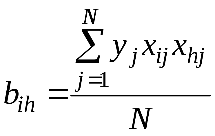 For (
For (  ), check hypothesisII– significance of coefficients for t-
Student's t test.
), check hypothesisII– significance of coefficients for t-
Student's t test.
 .
.
From the table we find  For
For  – number of degrees of freedom and significance level
q.
Number of duplicate experiments ( k) in the general case is equal to N.
– number of degrees of freedom and significance level
q.
Number of duplicate experiments ( k) in the general case is equal to N.
If
 , then the model coefficients are significant.
If
 ,
then the model coefficients are insignificant, i.e.
,
then the model coefficients are insignificant, i.e.  .
.
Statistical insignificance of model coefficients b i may be due to the following reasons:
– level of the basic value of the factor x i 0 close to the partial extremum point for the variable x i ;
– variation interval  small;
– factor x i does not affect the output parameter y(erroneously included in the experiment);
– the experimental error is large due to the presence of uncontrollable factors.
Let's write the model only with significant coefficients:
IIIhypothesis– adequacy of the model.
The hypothesis about the equality (homogeneity) of two variances is tested. The variance of adequacy is calculated using the formula:
 ,
,
Where d – number of significant coefficients of the model;
 – the value of the output parameter calculated by the model. To calculate
  x i
And x ih
corresponding to the first row of the matrix. To calculate
x i
And x ih
corresponding to the first row of the matrix. To calculate  substitute values into the model with significant coefficients x i
And x ih
corresponding to the second row of the matrix, etc.
substitute values into the model with significant coefficients x i
And x ih
corresponding to the second row of the matrix, etc.
The model is adequate to the experimental results if the condition is met
 .
.
 – determined from the table for
  ,
, and level of significance q.
The model is inadequate to the experimental results if:
– the form of the approximating polynomial is not suitable;
– large range of variation;
– the experimental error is large due to the presence of uncontrollable factors or significant factors are not included in the experiment.
Planning extreme experiments
Steep ascent method
Object of study – RES: amplifier, generator, power source.
As an example, we take an amplifier (Figure 42).
Steep Ascent Method Procedure(Q.30)
1 Centered at origin (base, zero)  We carry out PFE for this:
a) determine the variation interval  for each factor and calculate the levels of factor variation (see Table 3.1);
b) build a PFE matrix N=2 n(see table 3.3);
c) we carry out PFE and measure the values of the output parameter y j ;
d) we carry out statistical processing of the experimental results (we check the first hypothesis about the reproducibility of the experiment);
e) calculate the linear coefficients of the model b 0 , b 1 , b 2 , b 3 and write the equation as a linear polynomial.
For example
We check the significance of the model coefficients and the adequacy of the model.
2 Write the gradient of the response function:
For the example given: .
3 Let us pose the problem of finding  .
.
Calculate the product  for each factor, where
  – relative value of the variation interval (Table 3.4).
Table 3.4 – Parameters for carrying out the steep ascent method
|
Parameter | |||
|
b i | |||
|
b i λ i | |||
|
λ i kv | |||
|
Rounded λ i kv | |||
|
|
 , kOhm
4 Find  and define the basic i th factor s
  .
.
In the example, the base factor  .
.
For the base factor we take a steep ascent step  .
.
5 We calculate the step of steep ascent using other factors using the formula
 ,
,
in the numerator b i comes with his sign.
 ;
;
 .
.
Rounding up  .
.
Let's convert the relative value of the steep ascent step into a natural value:
 .
.
6 “We go” in the direction of the maximum (extremum) along the gradient.
To do this, you need to conduct experiments at new points on the plan.
First we carry out “mental” experiments. “Mental” experiments consist of calculating “predicted” values of the output parameter  at certain points
  factor space.
For this:
a) we calculate the values of factors in “mental” experiments using the formula
 ,
,
Where h = 1, 2, …, f–number of the steep ascent step (Table 3.5);
Table 3.5 – “Steps” of a steep ascent
|
N+ h |
Step number ( h) |
|
|
|


b) we encode the values of the factors for “mental” experiments and enter them into table 3.6:
 ;
;
 ;
;
 ;
;
 ;
;
 ;
;
 ;
;
 ;
;
 ;
;
 ;
;
 ;
;
Table 3.6 – Values of coded factors
|
N+ h |
x 2 |
|
||
|
|
||||
|
|
||||
|
|


c) substituting the coded values of the factors into the equation
 ,
,
calculate the output parameter  (
( ,
, do not calculate, they are in the PFE).
Let's count  ,
,
 ,
,
 for the example model:
7 We compare the results of “mental” experiments with the results of the experiment.
Choose  , corresponding to ( N+
h) “mental” experience.
, corresponding to ( N+
h) “mental” experience.
We check on the object of study (amplifier)  (point with parameters
  ).
).
We accept the terms ( N+ h)-th experience for the center of the new PFE (base point).
For example, for  =
= –
–
 kOhm;
kOhm;  kOhm;
kOhm;  kOhm
kOhm
8 We carry out PFE and statistical processing of the results. We find a new model (with different coefficients) and repeat the movement towards the optimum.
Since each cycle brings us closer to the optimum, we need to reduce the step  , or 0.01.
The movement towards the optimum is stopped when all the coefficients of the model are  .
.
Simplex optimization method (question 31)
The main feature of the simplex method of searching for an extremum is the combination of the processes of studying the response surface and moving along it. This is achieved by the fact that experiments are carried out only at points of the factor space corresponding to the vertices of the simplex.
The plan is based not on a hypercube used for PFE, but on a simplex - the simplest geometric figure, with a given number of factors.
What is simplex?
n-dimensional simplex is a convex figure formed by ( n+ 1)th points (vertices) that do not simultaneously belong to any ( n– 1)-dimensional subspace n-dimensional space ( X n).
For two factors x 1 and x 2 (n=2) a two-dimensional simplex looks like a triangle on a plane (Figure 44).

Figure 44 – Two-dimensional simplex with three vertices
For three factors x 1 , x 2 and x 3 (n=3) a three-dimensional simplex looks like a triangular pyramid (Figure 45).

Figure 45 – Three-dimensional simplex with four vertices
For one factor x 1 (n=1) a one-dimensional simplex has the form of a segment on a straight line (Figure 46).
Figure 46 – One-dimensional simplex with two vertices
The use of a simplex is based on its property, which is that by discarding one of the vertices with the worst result and using the remaining face, you can get a new simplex by adding one point that is a mirror of the discarded one. An experiment is placed at the vertices of the simplex, then a point with the minimum value of the output parameter ( y j) are discarded and a new simplex is built with a new vertex - a mirror image of the discarded one. A chain of simplices is formed, moving along the response surface to the extremum region (Figure 47).

Figure 47 – Movement towards the optimum along the response surface
To simplify calculations, we accept the condition that all edges of the simplex are equal.
If one of the vertices of the simplex is placed at the origin of coordinates, and the rest are positioned so that the edges emerging from this vertex form equal angles with the corresponding coordinate axes (Figure 48), then the coordinates of the vertices of the simplex can be represented by a matrix.

Figure 48 – Two-dimensional simplex with a vertex at the origin
Matrix of coordinates of vertices of a multidimensional simplex

If the distance between vertices is 1, then
 ;
;
 .
.
Sequential simplex procedure
1 Let you need to find  ,
,
2 Sets the variation step  for each factor x i. Example in table 3.7.
Table 3.7 – Factor values for the initial simplex
|
Parameter |
x i |
|
|
|
x 2 | |||
|
x 3 |


3 Sets the size of the simplex (distance between vertices)  regular simplex.
4 The vertices of the simplex are designated WITH j, Where j– vertex number. In the example j=4.
5 The initial simplex is oriented. To do this, one of the vertices of the initial simplex ( WITH j 0 ) is placed at the origin. Namely, the nominal values of the factors are taken as the zero point of the initial simplex.
A matrix of coordinates of the vertices of the simplex is constructed with the first vertex at the origin and the coordinate values of the vertices are entered into the table (Table 3.8).
Table 3.8 – Coordinates of the vertices of the simplex
|
Vertex coordinates |
|||||
|
x i |
x n |
||||
Calculate the coordinates of the remaining vertices of the initial simplex ( WITH j 0 ):
The calculation results are entered into the table (Table 3.9).
Table 3.9 – Coordinates of vertices and experiment results
|
simplex (WITH j0) |
Vertex coordinates |
y j |
|||
|
x 11 =x 10 |
x 21 =x 20 |
x 31 =x 30 | |||
|
y 2 |
|||||
|
WITH j * |
x 1 j * |
x 2 j * |
x 3 j * |
y j * |
|
The coordinate values of the vertices are calculated using formulas. For example n=3 we have:
 ;
;
 ;
; ;
;
 ;
;
 ;
; ;
;
 ;
;
 ;
; .
.
6 The experiment is being implemented at the vertices of the simplex.
To do this, set the values of the factors corresponding to the first vertex of the initial simplex WITH 10, and measure the values of the output parameter at 1 . Set the values of the factors corresponding to the second vertex WITH 20, and measure at 2 .
The factor values calculated for the example, corresponding to the coordinates of the vertices, are given in Table 3.10.
Table 3.10 – Factor values at the vertices of the simplex
|
simplex (WITH j0) |
Vertex coordinates |
y j |
|||
|
y 1 (5V) |
|||||
|
y 2 (6V) |
|||||
|
y 3 (4 IN) |
|||||
|
y 4 (8V) |
|||||
|
y 3 *(9V) |
|||||
|
y 1 *(5V) |
|||||
Calculation of vertex coordinates for n=3:
 ,
,

WITH 20 X 12 = 10+0.95∙2=11.9 kOhm;
X 22 = 3.0+0.24∙0.6=3.144 kOhm;
X 32 = 100+0.24∙20=104.8 kOhm;
WITH 30 X 13 = 10+0.24∙2=10.48 kOhm;
X 23 = 3.0+0.95∙0.6=3.57 kOhm;
X 33 = 100+0.24∙20=104.8 kOhm;
WITH 40 X 14 = 10+0.24∙2=10.48 kOhm;
X 24 = 3.0+0.24∙0.6=3.144 kOhm;
X 34 = 100+0.95∙20=119 kOhm.
7 Compare the values of the output parameter and discard the vertex corresponding to the minimum value y.
8 Calculate the coordinates of the new vertex of the mirror image of the worst point (“star point”) using the formula
Where  – coordinate designation j-th vertex (point), i=1,2,…,n– factor number, j=1,2,…,
(n+1) – number of the vertex of the simplex.
– coordinate designation j-th vertex (point), i=1,2,…,n– factor number, j=1,2,…,
(n+1) – number of the vertex of the simplex.
In the example  B is the minimum value, therefore the mirror point will be
  . For it, the vertex coordinates are calculated as:
9 Conduct an experiment at a new vertex WITH 3 * new simplex (C 10, WITH 20 , WITH 3 *, WITH y 3 *.
10 Compare the values of the output parameter of the new simplex ( y 1 , y 2 , y 3 *, at 4) and discard vertices with minimal y(For example y 1 =5V). We build a new simplex with a new vertex WITH 1 *.
To do this, calculate the coordinates of the vertex:

Conducting the experiment again at a new vertex WITH* 1 new simplex (C 1 *, WITH 20 , WITH 3 *, WITH 40) and measure the value of the output parameter y 1 *.
Comparing points with output parameters y 1 *=5, y 2 =6, y 3 * =9, y 4 =8. Discard the vertex with the minimum y 1 *=5. And again we determine a new “star point”.
The movement towards the optimum is stopped if the simplex begins to rotate, i.e. the same vertex occurs in more than ( n+1) successive simplexes.
11 Finally, PFE and statistical processing of the results are carried out. Find a model. The movement towards the optimum is stopped when all the coefficients of the model are  .
.
Technical task (TK, terms of reference)(question 8) - the source document for the design of a structure or industrial complex, the design of a technical device (device, machine, control system, etc.), the development of information systems, standards, or carrying out scientific research work (R&D).
The technical specification contains the basic technical requirements for a structure, product or service and the initial data for development; the technical specification indicates the purpose of the object, its scope, the stages of development of design (design, technological, software, etc.) documentation, its composition, deadlines, etc., as well as special requirements due to the specifics of the object itself or its conditions operation. As a rule, technical specifications are compiled based on an analysis of the results of preliminary studies, calculations and modeling.
As a communication tool in the customer-executor communication link, the terms of reference allow you to:
present the finished product
perform a point-by-point check of the finished product (acceptance testing - carrying out tests)
reduce the number of errors associated with changing requirements as a result of their incompleteness or error (at all stages and stages of creation, with the exception of tests)
realize what exactly he needs
require the contractor to comply with all the conditions specified in the technical specifications
understand the essence of the task, show the customer the “technical appearance” of the future product, software product or automated system
plan the implementation of the project and work according to the plan
refuse to perform work not specified in the technical specifications
both sides
to the customer
to the performer
Terms of Reference - the original document defining the procedure and conditions for carrying out work under the Contract, containing the purpose, objectives, principles of implementation, expected results and deadlines for completing the work.
The terms of reference are the fundamental document of the entire project and all relationships between the customer and the developer. Correct technical specifications, written and agreed upon by all interested and responsible persons, are the key to successful implementation of the project.
Question 9.
|
Development stage |
Stages of work execution |
|
Technical Proposal |
Selection of materials. Development of a technical proposal with the assignment of the letter “P” to documents. Review and approval of the technical proposal |
|
Preliminary design |
Development of a preliminary design with the assignment of the letter “E” to documents. Manufacturing and testing of mock-ups (if necessary) Review and approval of the preliminary design. |
|
Technical project |
Development of a technical project with the assignment of the letter “T” to documents. Manufacturing and testing of mock-ups (if necessary). Review and approval of the technical design. |
|
Detailed design documentation: a) a prototype (pilot batch) of a product intended for serial (mass) or single production (except for one-time production) |
Development of design documentation intended for the manufacture and testing of a prototype (pilot batch), without assigning a letter. Manufacturing and preliminary testing of a prototype (pilot batch). Correction of design documentation based on the results of manufacturing and preliminary testing of a prototype (pilot batch) with the assignment of the letter “O” to the documents. Acceptance tests of a prototype (pilot batch). Correction of design documentation based on the results of acceptance tests of a prototype (pilot batch) with assignment of the letter “O 1” to the documents. For a product developed by order of the Ministry of Defense, if necessary, - re-manufacture and testing of a prototype (pilot batch) according to the documentation with the letter “O 1” and adjustment of design documents with the assignment of the letter “O 2”. |
|
b) serial (mass) production |
Manufacturing and testing of the installation series according to the documentation with the letter “O 1” (or “O 2”). Correction of design documentation based on the results of manufacturing and testing of the installation series, as well as the equipment of the technological process of product manufacturing, with the assignment of the letter “A” to the design documents. For a product developed by order of the Ministry of Defense, if necessary, - production and testing of the lead (control) series according to documentation with the letter “A” and the corresponding adjustment of documents with the assignment of the letter “B” |
The mandatory implementation of stages and phases of development of design documentation is established by the technical specifications for development.
Notes: 1. The “Technical Proposal” stage does not apply to the design documentation of products developed by order of the Ministry of Defense. 2. The need to develop documentation for the manufacture and testing of prototypes is established by the developer. 3. Design documentation for the manufacture of prototypes is developed for the purpose of: checking the principles of operation of the product or its components at the preliminary design stage; checking the main design solutions of the product being developed or its components at the technical design stage; preliminary verification of the feasibility of changing individual parts of the manufactured product before introducing these changes into the working design documents of the prototype (pilot batch). 4. One-time production means the simultaneous production of one or more copies of a product, the further production of which is not envisaged.
2. Working design documents for single-production products intended for one-time production are assigned the letter “I” during their development, which may be preceded by the implementation of individual stages of development (technical proposal, preliminary design, technical design) and, accordingly, the stages of work indicated in the table.
1, 2. (Changed edition, Amendment No. 1).
3. (Deleted, Amendment No. 1).
4. Technical Proposal- a set of design documents that must contain technical and feasibility studies for the feasibility of developing product documentation based on an analysis of the customer’s technical specifications and various options for possible product solutions, a comparative assessment of solutions taking into account the design and operational features of the developed and existing products, and patent research.
The technical proposal, after coordination and approval in the prescribed manner, is the basis for the development of a preliminary (technical) design. Scope of work - according to GOST 2.118-73.
5. Preliminary design- a set of design documents that must contain fundamental design solutions that give a general idea of the structure and operating principle of the product, as well as data defining the purpose, main parameters and overall dimensions of the product being developed.
The preliminary design, after coordination and approval in the prescribed manner, serves as the basis for the development of a technical project or working design documentation. Scope of work - according to GOST 2.119-73.
6. Technical project- a set of design documents that must contain final technical solutions that give a complete picture of the structure of the product being developed, and the initial data for the development of working documentation.
The technical design, after coordination and approval in the prescribed manner, serves as the basis for the development of working design documentation. Scope of work - according to GOST 2.120-73. 7. Previously developed design documents are used when developing new or modernizing manufactured products in the following cases:
a) in design documentation (technical proposal, preliminary and technical designs) and working documentation of a prototype (pilot batch) - regardless of the lettering of the documents used;
b) in the design documentation with the letters “O 1” (“O 2”), “A” and “B”, if the lettering of the document used is the same or higher.
The lettering of a complete set of design documentation is determined by the lowest of the letters specified in the documents included in the set, except for documents of purchased products.
(Changed edition, Amendment No. 1).
8. Design documents, the holders of the originals of which are other enterprises, can only be used if there are registered copies or duplicates.
Systematic approach (issue 10) - this is the direction of studying an object from different sides, comprehensively, in contrast to previously used ones (physical, structural, etc.). With a systems approach within the framework of system modeling, it is necessary first of all to clearly define the purpose of the modeling. It must be remembered that it is impossible to completely simulate a really functioning system (original system), but it is necessary to create a model (model system) for the problem posed when solving a specific problem. Ultimately, modeling should adequately reflect the real processes of behavior of the systems under study. One of the goals of modeling is its cognitive orientation. The fulfillment of this goal is facilitated by the correct selection of system elements, structure and connections between them, and criteria for assessing the adequacy of the model into the created model. This approach simplifies the classification of real systems and their models.
Thus, in general, the systematic approach involves the following stages of solving the problem:
Study of the subject area (qualitative analysis).
Identifying and formulating the problem.
Mathematical (quantitative) formulation of the problem.
Full-scale and/or mathematical modeling of the objects and processes under study.
Statistical processing of simulation results.
Search and evaluation of alternative solutions.
Formulation of conclusions and proposals for solving the problem.
Question 17Requirements for ES designs and indicators of their quality When solving problems of designing custom LSIs and microwave IC crystals, the tasks of input control of source data, coating, layout, relative arrangement of components with a minimum number of intersections, routing, topology control, production of photomask designs and their originals are solved. The main thing that should be noted is that a radio engineer-designer-technologist is a user of computer technology, and not their developer and programmer, so he needs the basics of this knowledge in order to competently solve his problems in automated design. The main requirements for ES designs include high quality energy-information (electrical) indicators, reliability, strength, rigidity, manufacturability, cost-effectiveness and serializability of the design with low material consumption and power consumption. Designs that meet these requirements must have a minimum mass m, volume V, power consumption P, failure rate l, cost C and development time T, must be vibration and impact resistant, operate in normal thermal conditions and have a yield percentage high enough for production suitable products. Indicators characterizing these qualities can be divided into the following groups: absolute (in absolute units), complex (dimensionless, generalized), specific (in specific values) and relative (dimensionless, normalized). Absolute indicators include the weight of the structure, its volume, power consumption, failure rate, cost and development time. Sometimes this group of indicators is called material (M) indicators, answering the question of what and how the device is made. The group of energy-informational parameters in these cases is called functional (F) indicators, which answer the question of why and what the device can do. From these two groups, more general quality indicators can be obtained, such as a complex indicator and specific quality indicators. A complex quality indicator is the sum of normalized private material indicators with their “weighting” coefficients, as coefficients of significance of this parameter on the total quality of the structure: K=j m m o +j V V o +j l l o +j P P o +j C C o +j T T o , ( 1) where m o , V o , l o , P o , C o , T o are normalized values of material parameters relative to those specified in the technical specifications or the ratio of these material parameters for different comparative design options, j m , j V , j l , j P , j C , j T – coefficients of significance of private material parameters, determined by the method of expert assessments; usually their value is chosen in the range from 0 to 1. Expression (1) shows that the smaller each of the material parameters, the higher the quality of the design for the same functional parameters. Significance coefficients are determined by a group of experts (preferably at least 30 people), who, depending on the purpose and object of installation of the RES, each assign one or another value of the significance coefficient to the parameters. Next, their assessment results are summed up, the average values and root-mean-square values of these coefficients are determined, the acceptable deviation fields are found and the “misses” of the experts are eliminated, which are excluded from the total and then the same data processing operations are repeated. As a result, the average, “reliable” values of these coefficients are obtained, and thus the equation for calculations itself. Specific indicators of the quality of a structure include specific coefficients of structures: packing density of elements in an area or volume, specific dissipation power in an area or volume (thermal stress of a structure), specific mass (density) of a structure, the amount of gas flow from the volume of a structure (degree of tightness), Specific coefficients evaluate the progress of the development of new designs in comparison with previous analogues and prototypes. They are expressed as k=M/F and for each type of radio device or box they have a specific expression for the dimension of the quantities. So for antenna devices, if we take mass as the main parameter for them, the specific coefficient k A = m/G [kg/unit of gain], where G is the antenna gain; for transmitting devices k per =m/P out [kg/W], where P out is the output power of the transmitter. Since transmitting devices are characterized by a large number of functional parameters (gain, noise figure, bandwidth, output power, etc.), the functional complexity and quality of functions performed for microassemblies can be assessed by the number of developed microassemblies (n SMEs), then k per = m/ n MSB [kg/MSB]. Similarly, you can calculate the specific coefficients in relation to other material parameters and obtain their values for comparison of analogues, expressed in [cm 3 /unit of gain], [cm 3 /W], [cm 3 /MSB], [rub/unit. gain], [RUB/W], [RUB/SME], etc. Such assessments are the most obvious and do not require proof of what is better and what is worse without any emotions. The packing density of elements in an area or volume is estimated by the following expressions g S =N/S and g V =N/V, where N is the number of elements, S and V are the area or volume they occupy, respectively. The number of elements is determined as N=N IC *n e +n ERE, where N IC is the number of ICs in the device, n e is the number of elements in one IC (crystal or case), n ERE is the number of mounted electrical radio elements in the design of a cell, block, racks. Packing density is the main indicator of the level of integration of structures of a particular level. So, if for semiconductor ICs with a crystal volume of 1 mm 3 and the number of elements in it equal to 40 units, g IC = 40 * 10 3 el/cm 3 , then at the level of a digital RES unit g b = 40 el/cm 3 . This happens due to the fact that the crystals are packaged, then the packaged ICs are placed on the board with a known gap, and when the FC is assembled into a block, additional gaps again appear between the FC package and the inner walls of the package. And the case itself has a volume (volume of the walls and front panel), in which there are no useful (circuit) elements. In other words, when moving from one layout level to another, loss (disintegration) of useful volume occurs. As will be discussed below, the disintegration coefficient is determined by the ratio of the total volume to the useful volume. For a digital type block, it is expressed asq V =V b /N IC *V IC, where V IC is the volume of one microcircuit (either unpackaged or packaged, depending on the design method). Taking this expression into account, we can write that g b = (N IS *n e)/(q V * N IS *V IS) =g IS / q V, (2) where g IS =n e / V IS – density packing elements into ICs. As shown above, in unpackaged digital ICs with a low degree of integration, this value is 40 thousand cells/cm 3 . When installing unpackaged ICs into a package, for example type IV, the volume increases by about 200 times, and when installing packaged ICs on a board and then arranging them in the volume of the package another 5 times, i.e. the total disintegration coefficient is already 10 3, and this results in g b = 40 el/cm 3, which is typical for third-generation digital-type RES units. From expression (2) it follows that the design of highly integrated digital devices requires the developer not only to use LSI and VLSI, but also a fairly compact layout. For designs of analog ECs, where there are no clearly defined regular structures of active elements, where their number becomes commensurate with or even less than the number of passive mounted ECs (usually one analog IC is “framed” by up to 10 passive elements: capacitors along with coils and filters), the volume disintegration coefficients increase even more (3…4 times). It follows from this that it is impossible to compare constructs of different levels of hierarchy and different in purpose and principle of operation, i.e. this quality indicator is not universal for all ES. In addition, we add that if in one compact design an IC with a low degree of integration (up to 100 elements per package) was used, and in another - a poorly configured one, but on an LSI, then it may turn out by this indicator that the second design is better, although it is clearly visible that she is worse. Therefore, in the case of using an element base of varying degrees of integration, comparison of structures in terms of layout density is unlawful. Thus, the packing density of elements in the volume of a structure is a valid assessment of the quality of the structure, but this criterion must be used for comparison competently and objectively. The specific dissipation power determines the thermal intensity in the volume of the structure and is calculated as P specific dissipation = P dissipation /V, where P dissipation @(0.8…0.9) P for digital regular structures. In analog, especially in receiving-amplifier cells and blocks, power dissipation and thermal stress are low and the thermal regime is usually normal and with a large margin for this parameter. This is usually not observed in digital devices. The higher the requirements for the speed of computing facilities, the greater the amount of power consumed, the higher the thermal intensity. For RES on unframed SMEs, this problem is even more aggravated, since the volume during the transition from the III to the IV generation decreases, as noted above, by 5...6 times. Therefore, in the designs of digital-type blocks on open-frame SMEs, the presence of powerful heat sinks (metal frames, copper printed busbars, etc.) is mandatory. In some cases, cooling systems are also used in on-board RES, the type of which is selected according to the criterion of specific power dissipation from the surface of the block (P¢ ud.rass =P rass /S, W/cm 2). For digital type III generation blocks, the permissible thermal intensity is 20...30 W/dm 3 under conditions of natural convection and when the case is overheated relative to the environment by no more than 40 °C, and for IV generation blocks it is about 40 W/dm 3 or more. The specific gravity of the structure is expressed as m¢=m/V. This parameter was previously considered the main criterion for assessing the quality of equipment, and then there was a conditional division of structures into “sinking REA” (m¢>1 g/cm 3) and “floating REA” (m¢<1 г/см 3). Если конструкция была тонущая, то считали, что она компактна и хорошо скомпонована (мало воздуха и пустот в корпусе). Однако с появление IV поколения конструкций РЭС, где преобладающей долей массы являлись металлические рамки и с более толстыми стенками корпус (для обеспечения требуемой жесткости корпуса при накачке внутрь его азота), даже плохо скомпонованные ячейки оказывались тонущими. И чем больше и впустую расходовался металл, тем более возрастал этот показатель, переставший отражать качество компоновки и конструкции в целом. Поэтому для сравнения качества конструкций по этому критерию отказались, но он оказался полезным для решения другой задачи, а именно, распределение ресурса масс в конструктивах. Величина истечения газа из объема конструкции оценивает степень ее герметичности и определяется как D=V г *р/t , (3) где V г - объем газа в блоке, дм 3 ; р – величина перепада внутреннего и внешнего давления (избыточного давления) в блоке, Па (1 Па=7,5 мкм рт.ст.); t - срок службы или хранения, с. Для блоков с объемом V г =0,15…0,2 дм 3 в ответственных случаях при выдержке нормального давления к концу срока службы (8 лет) требуется D=6,65*10 -6 дм 3 *Па/с (или 5,5*10 -5 дм 3 *мкм рт.ст/с), в менее ответственных случаях полная вакуумная герметизация не обеспечивается и степень герметичности может быть уменьшена до значения 10 -3 дм 3 *мкм.рт.ст/с. В группе относительных показателей находятся коэффициенты дезинтеграции объема и массы, показатель функционального расчленения, величина перегрузки конструкции при вибрациях и ударах, а также многие параметры технологичности конструкции такие, как коэффициенты унификации и стандартизации, коэффициент повторяемости материалов и изделий электронной техники, коэффициент автоматизации и механизации и др. Последние достаточно хорошо известны из технологических дисциплин, поэтому повторять их содержание и влияние на качество конструкции не станем. Как уже отмечалось выше при рассмотрении плотности упаковки, в конструкциях РЭС разного уровня компоновки присутствуют потери полезного объема, а следовательно, и масс при корпусировании ИС, компоновке их в ячейки и далее в блоки, стойки. Уровень их может быть весьма значительным (в десятки и сотни раз). Оценки этих потерь (дезинтеграции) объемов и масс проводится с помощью коэффициентов дезинтеграции q V и q m соответственно, выражаемые как отношение суммарного объема (массы) конструктива к его полезному объему (массе), или q V =V/V N , q m =m/m N , (4) где V N =SV с.э., m N =Sm с.э. – полезный объем и масса схемных элементов. При переходе с одного уровня компоновки на более высший уровень коэффициенты дезинтеграции объема (или массы) q V(m) показывают, во сколько раз увеличиваются суммарные объем (или масса) комплектующих изделий к следующей конкретной форме их компоновки, например при переходе от нулевого уровня – корпусированных микросхем к первому – функциональной ячейке имеемq V(m) =V(m) ФЯ /SV(m) ИС, при переходе от уровня ячейки к блоку q V(m) = V(m) б /SV(m) ФЯ и т.д., где V(m) ИС, V(m) ФЯ, V(m) б – соответственно объемы (или массы) микросхемы, ячейки, блока. Как и в случае критерия плотности упаковки заметим, что коэффициенты дезинтеграции реально отражают качество конструкции, в частности ее компактность, но и они не могут быть использованы для сравнения конструктивов, если они относятся к разным поколениям, разным уровням конструктивной иерархии или ЭС различного назначения и принципа действия. Анализ существующих наиболее типовых и компактных конструктивов различных поколений и различного назначения позволил получить средние значения их коэффициентов дезинтеграции объема и массы (табл. 1). там же приведены значения удельной массы конструктивов. Показатель функционального разукрупнения конструкции представляет собой отношение количества элементов N в конструктиве к количеству выводов М из него, или ПФР=N/M. Например для цифровой бескорпусной МСБ, содержащей 12 бескорпусных ИС с 40 элементами в каждом кристалле (N=40*12=480 элементов) и 16 выходными площадками, имеем ПФР=480/16=30. Чем выше ПФР, тем ближе конструкция к конструктиву высокой интеграции, тем меньше монтажных соединений между ними, тем выше надежность и меньше масса и габариты. Наибольшее число функций и элементов монтажа "вбирают" в себя БИС¢ы и СБИС¢ы. Однако и у них есть предел степени интеграции, оговариваемый именно количеством допустимых выводов от активной площади кристалла к периферийным контактным площадкам. Наконец, величина перегрузки n действующих на конструкцию вибраций или ударов оценивается как отношение возникающего от их действия ускорения масс элементов конструкции к ускорению свободного падения, или n=a/g, где а – величина ускорения при вибрации (или ударе). Вибро- и ударопрочность конструкции определяются значениями величин допускаемых перегрузок при вибрациях и ударах, которые может выдержать конструкция без разрушения своих связей между элементами. Для того, чтобы эти свойства были обеспечены, необходимо, чтобы реально возникающие в тех или иных условиях эксплуатации перегрузки не превышали предельно допустимых для конкретной конструкции.
Question 26
Experimental planning is the selection of an experimental plan that meets specified requirements, a set of actions aimed at developing an experimentation strategy (from obtaining a priori information to obtaining a workable mathematical model or determining optimal conditions). This is purposeful control of an experiment, implemented under conditions of incomplete knowledge of the mechanism of the phenomenon being studied.
In the process of measurements, subsequent data processing, as well as formalization of the results in the form of a mathematical model, errors arise and some of the information contained in the original data is lost. The use of experimental planning methods makes it possible to determine the error of the mathematical model and judge its adequacy. If the accuracy of the model turns out to be insufficient, then the use of experimental planning methods makes it possible to modernize the mathematical model with additional experiments without losing previous information and with minimal costs.
The purpose of planning an experiment is to find such conditions and rules for conducting experiments under which it is possible to obtain reliable and reliable information about an object with the least amount of labor, as well as to present this information in a compact and convenient form with a quantitative assessment of accuracy.
Let the property (Y) of an object that interests us depend on several (n) independent variables (X1, X2, ..., Xn) and we want to find out the nature of this dependence - Y=F(X1, X2, ..., Xn), about which we have just a general idea. The value Y is called the “response”, and the dependence Y=F(X1, X2, …, Xn) itself is called the “response function”.
The response must be quantified. However, there may also be qualitative characteristics of Y. In this case, it is possible to use the rank approach. An example of a ranking approach is an assessment in an exam, when a complex set of information obtained about a student’s knowledge is assessed with a single number.
Independent variables X1, X2, ..., Xn - otherwise factors, must also have a quantitative assessment. If qualitative factors are used, then each level should be assigned a number. It is important to select only independent variables as factors, i.e. only those that can be changed without affecting other factors. The factors must be clear. To build an effective mathematical model, it is advisable to conduct a preliminary analysis of the significance of factors (the degree of influence on the function), their ranking, and eliminate unimportant factors.
The ranges of variation of factors determine the domain of definition of Y. If we assume that each factor has a corresponding coordinate axis, then the resulting space is called factor space. For n=2, the domain of definition of Y is a rectangle, for n=3 it is a cube, and for n >3 it is a hypercube.
When choosing ranges for changing factors, their compatibility must be taken into account, i.e. control that in these ranges any combinations of factors are feasible in experiments and do not lead to absurdity. For each factor, limit values are indicated
![]() , i=1,...n.
, i=1,...n.
Regression analysis of the response function is intended to obtain its mathematical model in the form of a regression equation
where B1, …, Bm are some coefficients; e – error.
Among the main planning methods used at different stages of the study are:
planning a screening experiment, the main meaning of which is the selection from the entire set of factors of a group of significant factors that are subject to further detailed study;
designing an experiment for analysis of variance, i.e. drawing up plans for objects with qualitative factors;
planning a regression experiment that allows obtaining regression models (polynomial and others);
planning an extreme experiment in which the main task– experimental optimization of the research object;
planning when studying dynamic processes, etc.
The initiator of the application of experimental design is Ronald A. Fisher, another author famous first works - Frank Yates. Further, ideas for planning an experiment were formed in the works of J. Box and J. Kiefer. In our country - in the works of G.K. Kruga, E.V. Markova and others.
Currently, experimental planning methods are embedded in specialized packages widely available on the software market, for example: StatGrapfics, Statistica, SPSS, SYSTAT, etc.
Question 18 Full factorial the experiment assumes the ability to control an object through one or several independent channels (see Fig. 1.5, c).
In general, the experimental design can be presented as shown in Fig. 1.5, c. The scheme uses the following groups of parameters:
1. managers (input)
2. status parameters(weekend )
3. disturbing influences ()
In a multifactorial and full factorial experiment, there may be several output parameters. An example of such a passive multifactorial experiment will be discussed in the sixth chapter of this book.
Control parameters are independent variables that can be changed to control output parameters. The control parameters are called factors. If (one control parameter), then the experiment is one-factor. A multivariate experiment corresponds to a finite number of control parameters. A full factorial experiment corresponds to the presence of disturbances in a multifactorial experiment.
The range of changes in factors or the number of values that they can take is called factor level.
A complete factorial experiment is characterized by the fact that, for fixed disturbances, the minimum number of levels of each factor is two. In this case, having fixed all the factors except for one, it is necessary to carry out two measurements corresponding to two levels of this factor. Consistently carrying out this procedure for each of the factors, we obtain the required number of experiments in a full factorial experiment to implement all possible combinations of factor levels, where is the number of factors.
1. The history of experimental planning
Experimental design is a product of our time, but its origins are lost in the mists of time.
The origins of experimental planning go back to ancient times and are associated with numerical mysticism, prophecies and superstitions.
This is actually not planning a physical experiment, but planning a numerical experiment, i.e. arrangement of numbers so that certain strict conditions are met, for example, the equality of the sums along the rows, columns and diagonals of a square table, the cells of which are filled with numbers from the natural series.
Such conditions are fulfilled in magic squares, which, apparently, have primacy in the planning of the experiment.
According to one legend, around 2200 BC. Chinese Emperor Yu performed mystical calculations using a magic square, which was depicted on the shell of a divine turtle.
Emperor Yu Square
The cells of this square are filled with numbers from 1 to 9, and the sum of the numbers in rows, columns and main diagonals is 15.
In 1514, the German artist Albrecht Durer depicted a magic square in the right corner of his famous allegory engraving “Melancholy”. The two numbers in the lower horizontal row A5 and 14) represent the year the engraving was created. This was a kind of “application” of the magic square.
Durer square
For several centuries, the construction of magic squares occupied the minds of Indian, Arab, German, and French mathematicians.
Currently, magic squares are used when planning an experiment under conditions of linear drift, when planning economic calculations and preparing food rations, in coding theory, etc.
The construction of magic squares is a task of combinatorial analysis, the foundations of which in its modern understanding were laid by G. Leibniz. He not only examined and solved basic combinatorial problems, but also pointed out the great practical application of combinatorial analysis: to encoding and decoding, to games and statistics, to the logic of inventions and the logic of geometry, to the art of war, grammar, medicine, law, technology, etc. combinations of observations. The last area of application is closest to experimental design.
One of the combinatorial problems, which is directly related to the planning of an experiment, was studied by the famous St. Petersburg mathematician L. Euler. In 1779, he proposed the problem of 36 officers as some kind of mathematical curiosity.
He posed the question whether it was possible to select 36 officers of 6 ranks from 6 regiments, one officer of each rank from each regiment, and arrange them in a square so that in each row and in each rank there would be one officer of each rank and one from each regiment . The problem is equivalent to constructing paired orthogonal 6x6 squares. It turned out that this problem cannot be solved. Euler suggested that there is no pair of orthogonal squares of order n=1 (mod 4).
Many mathematicians subsequently studied Euler's problem, in particular, and Latin squares in general, but almost none of them thought about the practical application of Latin squares.
Currently, Latin squares are one of the most popular methods of limiting randomization in the presence of discrete-type sources of inhomogeneity in experimental design. Grouping the elements of a Latin square, due to its properties (each element appears once and only once in each row and in each column of the square), allows you to protect the main effects from the influence of the source of inhomogeneities. Latin squares are also widely used as a means of reducing enumeration in combinatorial problems.
The emergence of modern statistical methods of experiment planning is associated with the name of R. Fisher.
In 1918, he began his famous series of works at the Rochemsted Agrobiological Station in England. In 1935, his monograph “Design of Experiments” appeared, which gave the name to the entire direction.
Among planning methods, the first was analysis of variance (by the way, Fisher also coined the term “variance”). Fisher created the basis of this method by describing complete ANOVA classifications (univariate and multivariate experiments) and partial ANOVA classifications without restriction and with restriction on randomization. At the same time, he made extensive use of Latin squares and flowcharts. Together with F. Yates, he described their statistical properties. In 1942, A. Kishen considered planning using Latin cubes, which was a further development of the theory of Latin squares.
Then R. Fischer independently published information about orthogonal hyper-Greco-Latin cubes and hyper-cubes. Soon after 1946–1947) R. Rao examined their combinatorial properties. The works of X. Mann (A947–1950) are devoted to the further development of the theory of Latin squares.
R. Fischer's research, carried out in connection with work on agrobiology, marks the beginning of the first stage in the development of experimental design methods. Fisher developed the factorial planning method. Yeggs proposed a simple computational scheme for this method. Factorial planning has become widespread. A feature of a full factorial experiment is the need to conduct a large number of experiments at once.
In 1945, D. Finney introduced fractional replicas from the factorial experiment. This allowed a sharp reduction in the number of experiments and paved the way for technical planning applications. Another possibility of reducing the required number of experiments was shown in 1946 by R. Plackett and D. Berman, who introduced saturated factorial designs.
In 1951, the work of American scientists J. Box and K. Wilson began a new stage in the development of experimental planning.
This work summarized the previous ones. It clearly formulated and brought to practical recommendations the idea of sequential experimental determination of optimal conditions for carrying out processes using the estimation of coefficients of power expansions using the method least squares, movement along the gradient and finding an interpolation polynomial (power series) in the region of the extremum of the response function (“almost stationary” region).
In 1954–1955 J. Box, and then J. Box and P. Yule showed that experimental design can be used in the study of physicochemical mechanisms of processes if one or more possible hypotheses are a priori stated. Here, experimental design intersected with chemical kinetics studies. It is interesting to note that kinetics can be considered as a method of describing a process using differential equations, the traditions of which go back to I. Newton. The description of a process by differential equations, called deterministic, is often contrasted with statistical models.
Box and J. Hunter formulated the principle of rotatability to describe the "nearly stationary" field, which is now developing into an important branch of the theory of experimental design. The same work shows the possibility of planning with partitioning into orthogonal blocks, previously indicated independently by de Baun.
A further development of this idea was planning orthogonal to uncontrolled time drift, which should be considered as important discovery in experimental technology - a significant increase in the capabilities of the experimenter.
2. Mathematical planning of experiments in scientific research
2.1 Basic concepts and definitions
By experiment we mean a set of operations performed on an object of study in order to obtain information about its properties. An experiment in which the researcher, at his discretion, can change the conditions of its conduct is called an active experiment. If the researcher cannot independently change the conditions of its conduct, but only registers them, then this is a passive experiment.
The most important task of methods for processing information obtained during an experiment is the task of constructing a mathematical model of the phenomenon, process, or object being studied. It can be used in process analysis and object design. It is possible to obtain a well-approximating mathematical model if an active experiment is purposefully used. Another task of processing the information obtained during the experiment is the optimization problem, i.e. finding such a combination of influencing independent variables that the selected optimality indicator takes an extreme value.
Experience is a separate experimental part.
Experimental plan – a set of data that determines the number, conditions and order of experiments.
Experimental planning is the selection of an experimental plan that meets specified requirements, a set of actions aimed at developing an experimentation strategy (from obtaining a priori information to obtaining a workable mathematical model or determining optimal conditions). This is purposeful control of an experiment, implemented under conditions of incomplete knowledge of the mechanism of the phenomenon being studied.
In the process of measurements, subsequent data processing, as well as formalization of the results in the form of a mathematical model, errors arise and some of the information contained in the original data is lost. The use of experimental planning methods makes it possible to determine the error of the mathematical model and judge its adequacy. If the accuracy of the model turns out to be insufficient, then the use of experimental planning methods makes it possible to modernize the mathematical model with additional experiments without losing previous information and with minimal costs.
The purpose of planning an experiment is to find such conditions and rules for conducting experiments under which it is possible to obtain reliable and reliable information about an object with the least amount of labor, as well as to present this information in a compact and convenient form with a quantitative assessment of accuracy.
Let the property we are interested in (Y) object depends on several ( n) independent variables ( X 1, X 2, …, X n) and we want to find out the nature of this dependence - Y=F(X 1, X 2, …, X n), about which we have only a general idea. Magnitude Y– is called “response”, and the dependence itself Y=F(X 1, X 2, …, X n)– “response function”.
The response must be quantified. However, there may also be qualitative signs Y. In this case, it is possible to use the rank approach. An example of a ranking approach is an assessment in an exam, when a complex set of information obtained about a student’s knowledge is assessed with a single number.
Independent Variables X 1, X 2, …, X n– otherwise the factors must also be quantified. If qualitative factors are used, then each level should be assigned a number. It is important to select only independent variables as factors, i.e. only those that can be changed without affecting other factors. The factors must be clear. To build an effective mathematical model, it is advisable to conduct a preliminary analysis of the significance of factors (the degree of influence on the function), their ranking, and eliminate unimportant factors.
The ranges of change of factors determine the area of definition Y. If we assume that each factor has a corresponding coordinate axis, then the resulting space is called factor space. For n=2, the domain of definition of Y is a rectangle, for n=3 it is a cube, and for n >3 it is a hypercube.
When choosing ranges for changing factors, their compatibility must be taken into account, i.e. control that in these ranges any combinations of factors are feasible in experiments and do not lead to absurdity. For each factor, limit values are indicated
, i =1,… n .
Regression analysis of the response function is intended to obtain its mathematical model in the form of a regression equation
Where V 1, …, V m– some coefficients; e– error.
Among the main planning methods used at different stages of the study are:
· planning a screening experiment, the main meaning of which is the selection from the entire set of factors of a group of significant factors that are subject to further detailed study;
· designing an experiment for analysis of variance, i.e. drawing up plans for objects with qualitative factors;
· planning a regression experiment that allows obtaining regression models (polynomial and others);
· planning an extreme experiment in which the main task is experimental optimization of the research object;
· planning when studying dynamic processes, etc.
The initiator of the use of experimental design is Ronald A. Fisher, another author of famous early works is Frank Yates. Further, ideas for planning an experiment were formed in the works of J. Box and J. Kiefer. In our country - in the works of G.K. Kruga, E.V. Markova and others.
Currently, experimental planning methods are embedded in specialized packages widely available on the software market, for example: StatGrapfics, Statistica, SPSS, SYSTAT, etc.
2.2 Presentation of experimental results
When using experimental design methods, it is necessary to find answers to 4 questions:
· What combinations of factors and how many such combinations must be taken to determine the response function?
· How to find odds V 0, V 1, …, B m ?
· How to evaluate the accuracy of the response function representation?
· How to use the resulting representation to find optimal values Y ?
Geometric representation of the response function in factor space X 1, X 2, …, X n called the response surface (Fig. 1).

Rice. 1. Response surface
If the influence on Y only one factor X 1, then finding the response function is enough simple task. Having given several values of this factor, as a result of experiments we obtain the corresponding values Y and schedule Y =F(X)(Fig. 2).

Rice. 2. Construction of the response function of one variable using experimental data
Based on its appearance, one can select a mathematical expression for the response function. If we are not sure that the experiments are well reproduced, then usually the experiments are repeated several times and a dependence is obtained taking into account the scatter of experimental data.
If there are two factors, then it is necessary to conduct experiments with different ratios of these factors. The resulting response function in 3-dimensional space (Fig. 1) can be analyzed by conducting a series of sections with fixed values of one of the factors (Fig. 3). Isolated cross-section graphs can be approximated by a set of mathematical expressions.

Rice. 3. Sections of the response surface for fixed responses (a) and variable responses (b, c)
With three or more factors, the problem becomes practically unsolvable. Even if solutions are found, it is quite difficult to use a set of expressions, and often not realistic.
2.3 Application of mathematical experimental planning in scientific research
In modern mathematical theory There are 2 main sections to optimal experimental planning:
1. planning an experiment to study mechanisms complex processes and properties of multicomponent systems.
2. planning an experiment to optimize technological processes and properties of multicomponent systems.
Experiment planning – This is the choice of the number of experiments and the conditions for their conduct necessary and sufficient to solve the problem with the required accuracy.
An experiment that is set up to solve optimization problems is called extreme. Examples of optimization problems are choosing the optimal composition of multicomponent mixtures, increasing the productivity of an existing installation, improving product quality and reducing the cost of obtaining it. Before planning an experiment, it is necessary to formulate the purpose of the study. The success of the study depends on the precise formulation of the goal. It is also necessary to make sure that the research object meets the requirements imposed on it. In technological research, the purpose of research when optimizing a process is most often to increase product yield, improve quality, and reduce costs.
The experiment can be carried out directly on the object or on its model. A model differs from an object not only in scale, but sometimes in nature. If the model accurately describes the object, then the experiment on the object can be transferred to the model. To describe the concept of “research object”, you can use the idea of a cybernetic system, which is called black box.


The arrows on the right depict the numerical characteristics of the research objectives and are called output parameters ( y ) or optimization parameters .
To conduct an experiment, it is necessary to influence the behavior of the black box. All methods of influence are denoted by “x” and are called input parameters or factors . Each factor can take one of several values in experience, and such values are called levels . A fixed set of levels and factors determines one of the possible states of the black box; at the same time, they are the conditions for conducting one of the possible experiments. The results of the experiment are used to obtain a mathematical model of the research object. Using every possible experiment on an object results in absurdly large experiments. In this regard, experiments must be planned.
The task of planning is to select the experiments necessary for the experiment, methods for mathematical processing of their results and decision-making. A special case of this problem is planning an extreme experiment. That is, an experiment carried out with the aim of finding optimal conditions for the functioning of an object. Thus, planning an extreme experiment is the choice of the number and conditions of experiments that are minimally necessary to find optimal conditions. When planning an experiment, the research object must have the following mandatory properties:
1.controlled
2.the results of the experiment must be reproducible .
The experiment is called reproducible , if under fixed experimental conditions the same yield is obtained within a given relatively small experimental error (2% -5%). The experiment is carried out by selecting certain levels for all factors, then it is repeated at irregular intervals. And the values of the optimization parameters are compared. The spread of these parameters characterizes the reproducibility of the results. If it does not exceed in advance given value, then the object satisfies the requirement of reproducibility of results.
When designing an experiment, active intervention involves a process and the ability to select in each experiment those factors that are of interest. An experimental study of the influence of input parameters (factors) on output parameters can be carried out using the method of passive or active experiment. If an experiment comes down to obtaining the results of observing the behavior of a system with random changes in input parameters, then it is called passive . If, during an experiment, the input parameters change according to a predetermined plan, then such an experiment is called active. An object on which an active experiment is possible is called manageable. In practice, there are no absolutely managed objects. A real object is usually affected by both controllable and uncontrollable factors. Uncontrollable factors affect the reproducibility of the experiment. If all factors are uncontrollable, the problem arises of establishing a connection between the optimization parameter and the factors based on the results of observations or the results of a passive experiment. Poor reproducibility of changes in factors over time is also possible.
3. Optimization parameters
3.1 Types of optimization parameters
Optimization parameter– this is a sign by which we want to optimize the process. It must be quantitative, given by number. The set of values that an optimization parameter can take is called its domain of definition. Areas of definition can be continuous and discrete, limited and unlimited. For example, the output of a reaction is an optimization parameter with a continuous limited domain. It can vary from 0 to 100%. The number of defective products, the number of blood cells in a blood sample are examples of parameters with a discrete definition range limited from below.
Depending on the object and purpose of the study, optimization parameters can be very diverse (Fig. 1).
Let us comment on some elements of the scheme. Economic optimization parameters, such as profit, cost and profitability, are usually used when studying existing industrial facilities, while it makes sense to evaluate the costs of an experiment in any research, including laboratory ones. If the price of the experiments is the same, the costs of the experiment are proportional to the number of experiments that need to be carried out to solve a given problem. This largely determines the choice of experimental design.
Among the technical and economic parameters, productivity is the most widespread. Parameters such as durability, reliability and stability are associated with long-term observations. There is some experience of using them in the study of expensive, critical objects, such as electronic equipment.
Almost all studies have to take into account the quantity and quality of the resulting product. Yield, for example, the percentage of finished product yield, is used as a measure of the amount of product.
Quality indicators are extremely varied. In our scheme they are grouped by property type. The characteristics of the quantity and quality of the product form a group of technical and technological parameters.
The “other” group groups various parameters that are less common, but no less important. This includes statistical parameters used to improve the characteristics of random variables or random functions.
3.2 Requirements for the optimization parameter
An optimization parameter is a sign by which we want to optimize the process. It must be quantitative, given by number. We must be able to measure it for any possible combination of selected factor levels. The set of values that an optimization parameter can take will be called its domain of definition. Areas of definition can be continuous and discrete, limited and unlimited. For example, the output of a reaction is an optimization parameter with a continuous limited domain. It can vary from 0 to 100%. The number of defective products, the number of grains on a thin section of an alloy, the number of blood cells in a blood sample - these are examples of parameters with a discrete definition range limited from below.
To be able to measure an optimization parameter means to have a suitable instrument. In some cases, such a device may not exist or it may be too expensive. If there is no way to quantify the result, then you have to use a technique called ranking (rank approach). In this case, the optimization parameters are assigned ratings - ranks on a pre-selected scale: two-point, five-point, etc. The rank parameter has a discrete limited domain of definition. In the simplest case, the area contains two values (yes, no; good, bad). This may correspond, for example, to good products and defective products.
Rank is a quantitative assessment of an optimization parameter, but it is conditional (subjective) in nature. We assign a certain number – rank – to a qualitative attribute. For each physically measured optimization parameter, a rank analogue can be constructed. The need to construct such an analogue arises if the numerical characteristics available to the researcher are inaccurate or the method for constructing satisfactory numerical estimates is unknown. All other things being equal, one should always give preference to the physical measurement, since the rank approach is less sensitive and with its help it is difficult to study subtle effects.
Example: A technologist has developed a new type of product. You need to optimize this process.
The goal of the process is to obtain a tasty product, but such a formulation of the goal does not yet make it possible to begin optimization: it is necessary to select a quantitative criterion that characterizes the degree of achievement of the goal. You can make the following decision: a very tasty product gets a mark of 5, a simply tasty product gets a mark of 4, etc.
Is it possible to move on to process optimization after such a decision? It is important for us to quantify the optimization result. Does marking solve this problem? Of course, because, as we agreed, mark 5 corresponds to a very tasty product, etc. Another thing is that this approach, called the rank approach, often turns out to be rude and insensitive. But the possibility of such a quantitative assessment of the results should not raise doubts.
The next requirement: the optimization parameter must be expressed as a single number. For example: recording instrument readings.
Another requirement related to the quantitative nature of the optimization parameter is unambiguity in a statistical sense. A given set of factor values must correspond to one optimization parameter value, accurate to within the experimental error. (However, the reverse is not true: different sets of factor values can correspond to the same parameter value.)
To successfully achieve the research goal, it is necessary that the optimization parameter truly evaluates the efficiency of the system in a pre-selected sense. This requirement is the main one that determines the correctness of the problem statement.
Perceptions of effectiveness do not remain constant throughout the study. It changes as information accumulates and depending on the results achieved. This leads to a consistent approach when choosing an optimization parameter. For example, in the first stages of process research, product yield is often used as an optimization parameter. However, in the future, when the possibility of increasing the yield has been exhausted, we begin to be interested in such parameters as cost, product purity, etc.
When talking about assessing the effectiveness of a system, it is important to remember that we are talking about the system as a whole. Often a system consists of a number of subsystems, each of which can be evaluated by its own local optimization parameter.
The next requirement for an optimization parameter is the requirement of universality or completeness. The universality of an optimization parameter is understood as its ability to comprehensively characterize an object. In particular, technological optimization parameters are not universal enough: they do not take into account economics. For example, generalized optimization parameters, which are constructed as functions of several particular parameters, are universal.
It is desirable that the optimization parameter has a physical meaning, is simple and easy to calculate.
The requirement for physical meaning is associated with the subsequent interpretation of the experimental results.
So the optimization parameter should be:
– effective in terms of achieving the goal;
– universal;
– quantitative and expressed in one number;
– statistically effective;
– having a physical meaning, simple and easy to calculate.
In cases where difficulties arise with the quantitative assessment of optimization parameters, one has to turn to the rank approach. During the course of the study, a priori ideas about the object of study may change, which leads to a consistent approach when choosing an optimization parameter.
Of the many parameters characterizing the object of study, only one, often generalized, can serve as an optimization parameter. The rest are considered restrictions.
4. Optimization factors
4.1 Definition of factor
factor is a measured variable that takes on a certain value at some point in time. Factors correspond to the ways of influencing the object of study.
Just like the optimization parameter, each factor has a domain of definition. A factor is considered given if the area of its definition is indicated along with its name.
Under domain of definition is understood as the totality of all values that a given factor can, in principle, take.
The set of factor values that is used in the experiment is a subset of the set of values that form the domain of definition. The domain of definition can be continuous or discrete. However, in general, in experimental planning problems, discrete domains of definition are used. Thus, for factors with a continuous domain of definition, such as temperature, time, amount of substance, etc., discrete sets of levels are always selected.
In practical problems, the scope of determining factors is usually limited. Restrictions may be of a fundamental or technical nature.
Factors are classified depending on whether the factor is a variable value that can be assessed quantitatively: measured, weighed, titrated, etc., or whether it is some variable characterized by qualitative properties.
Factors are divided into quantitative and qualitative.
Qualitative factors– these are different substances, different technological methods, devices, performers, etc.
Although qualitative factors do not correspond to a numerical scale in the sense that is understood for quantitative factors, it is possible to construct a conditional ordinal scale that matches the levels of the qualitative factor with numbers in the natural series, i.e. does the coding. The order of levels can be arbitrary, but after encoding it is fixed.
Qualitative factors do not have a numerical scale, and the order of factor levels does not matter.
Reaction time, temperature, concentration of reactants, feed rate of substances, pH value are examples of the most frequently encountered quantitative factors. Various reagents, adsorbents, vulcanizing agents, acids, metals are examples of the levels of quality factors.
4.2 Requirements for factors when planning an experiment
When designing an experiment, factors must be controllable. This means that the experimenter, having chosen the desired value of the factor, can maintain it constant throughout the experiment, i.e. can control the factor. An experiment can only be planned if the levels of factors are subject to the will of the experimenter.
Example: You are studying the process of ammonia synthesis. The synthesis column is installed in an open area. Is air temperature a factor that can be included in experimental design?
Air temperature is an uncontrollable factor. We have not yet learned how to make the weather to order. And only those factors that can be controlled can participate in planning - set and maintained at a selected level during the experiment or changed according to a given program. In this case, it is impossible to control the ambient temperature. It can only be controlled.
To accurately determine a factor, you need to indicate the sequence of actions (operations) by which its specific values (levels) are established. We will call this definition of a factor operational. Thus, if the factor is the pressure in some apparatus, then it is absolutely necessary to indicate at what point and with what instrument it is measured and how it is set. The introduction of an operational definition provides an unambiguous understanding of the factor.
The operational definition is associated with the choice of factor dimension and the accuracy of its recording.
The accuracy of factor measurement should be as high as possible. The degree of accuracy is determined by the range of changes in factors. When studying a process that lasts tens of hours, there is no need to take into account fractions of a minute, but in fast processes it is necessary to consider, perhaps, fractions of a second.
Factors must be direct impacts on the object. The factors must be clear. It is difficult to control a factor that appears to be a function of other factors. But complex factors may be involved in planning, such as relationships between components, their logarithms, etc.
When designing an experiment, several factors are usually changed simultaneously. Therefore, it is very important to formulate the requirements that apply to a combination of factors. First of all, the requirement of compatibility is put forward. The compatibility of factors means that all their combinations are feasible and safe. This is a very important requirement.
When planning an experiment, the independence of factors is important, i.e. the ability to establish a factor at any level, regardless of the levels of other factors. If this condition is not met, then it is impossible to plan the experiment.
Thus, it was established that factors are variable quantities corresponding to the ways in which the external environment influences an object.
They define both the object itself and its state. Requirements for factors: controllability and unambiguity.
To control a factor means to set the desired value and maintain it constant during the experiment or change it according to a given program. This is the peculiarity of the “active” experiment. An experiment can only be planned if the levels of factors are subject to the will of the experimenter.
Factors must directly affect the object of study.
Requirements for a set of factors: compatibility and lack of linear correlation. The selected set of factors should be sufficiently complete. If any essential factor is omitted, it will lead to incorrect determination of optimal conditions or to large experimental error. Factors can be quantitative or qualitative.
5. Experimental errors
It is impossible to simultaneously study all the factors influencing the object under study; therefore, the experiment considers a limited number of them. The remaining active factors stabilize, i.e. are established at some levels that are the same for all experiments.
Some factors cannot be provided by stabilization systems (for example, weather conditions, the operator’s well-being, etc.), while others are stabilized with some error (for example, the content of a component in the medium depends on the error when taking the sample and preparing the solution ). Considering also that the measurement of the parameter at carried out by a device that has some kind of error depending on the accuracy class of the device, we can come to the conclusion that the results of repetitions of the same experiment y k will be approximate and must differ from one another and from the true value of the process output. Uncontrolled, random changes and many other factors influencing the process cause random deviations of the measured value y k from its true meaning - an error of experience.
Each experiment contains an element of uncertainty due to the limited experimental material. Conducting repeated (or parallel) experiments does not give completely identical results, because there is always an experimental error (reproducibility error). This error must be assessed using parallel experiments. To do this, the experiment is reproduced, if possible, under the same conditions several times and then the arithmetic mean of all the results is taken. The arithmetic mean y is equal to the sum of all n individual results divided by the number of parallel experiments n:

The deviation of the result of any experiment from the arithmetic mean can be represented as the difference y 2 – , where y 2 is the result of a separate experiment. The presence of a deviation indicates variability, variation in the values of repeated experiments. Variance is most often used to measure this variability.
Dispersion is the average value of the squared deviation of a value from its mean value. The variance is denoted by s 2 and is expressed by the formula:

where (n-1) is the number of degrees of freedom equal to the number of experiments minus one. One degree of freedom is used to calculate the average.
The square root of the variance, taken with a positive sign, is called the standard deviation, standard or square error:

The experimental error is a total value, the result of many errors: errors in measuring factors, errors in measuring optimization parameters, etc. Each of these errors can, in turn, be divided into components.
All errors are usually divided into two classes: systematic and random (Figure 1).
Systematic errors are generated by causes that act regularly in a certain direction. More often than not, these errors can be studied and quantified. Systematic error – this is an error that remains constant or changes naturally with repeated measurements of the same quantity. These errors appear due to malfunction of the instruments, inaccuracy of the measurement method, some omission by the experimenter, or the use of inaccurate data for calculations. Detecting systematic errors and eliminating them in many cases is not easy. A thorough analysis of analysis methods, strict checking of all measuring instruments and unconditional implementation of practice-developed rules are required. experimental work. If systematic errors are caused by known causes, then they can be identified. Such errors can be eliminated by introducing corrections.
Systematic errors are found by calibrating measuring instruments and comparing experimental data with changing external conditions (for example, when calibrating a thermocouple using reference points, when comparing with a reference device). If systematic errors are caused by external conditions (variable temperature, raw materials, etc.), their influence should be compensated.
Random Errors are those that appear irregularly, the causes of which are unknown and which cannot be taken into account in advance. Random errors are caused by both objective and subjective reasons. For example, imperfection of instruments, their lighting, location, temperature changes during measurements, contamination of reagents, changes in electric current in the circuit. When the random error is greater than the instrument error, it is necessary to repeat the same measurement many times. This makes it possible to make a random error comparable to the error introduced by the device. If it is less than the instrument error, then there is no point in reducing it. Such errors have meanings that differ in individual measurements. Those. their values may not be the same for measurements made even under the same conditions. Since the reasons leading to random errors are not the same in each experiment and cannot be taken into account, therefore random errors cannot be excluded, one can only estimate their values. When determining any indicator multiple times, you may encounter results that differ significantly from other results in the same series. They may be the result of a gross error caused by the inattention of the experimenter.
Systematic and random errors consist of many elementary errors. In order to exclude instrumental errors, instruments should be checked before the experiment, sometimes during the experiment, and always after the experiment. Errors during the experiment itself arise due to uneven heating of the reaction medium, different stirring methods, etc.
When repeating experiments, such errors can cause a large scatter of experimental results.
It is very important to exclude from the experimental data gross errors, the so-called defects in repeated experiments. Gross mistakes easy to detect. To identify errors, it is necessary to make measurements under other conditions or repeat measurements after some time. To prevent gross errors, you need to be careful in your notes, thorough in your work and recording the results of the experiment. The gross error must be excluded from the experimental data. There are certain rules for discarding erroneous data.
For example, the Student t-criterion t(P; f) is used: The experiment is considered defective if the experimental value of the t-criterion is greater in absolute value than the tabulated value t(P; f).
If the researcher has at his disposal an experimental estimate of the variance S 2 (y k) with a small finite number of degrees of freedom, then the confidence errors are calculated using the Student t criterion t(P; f):
ε() = t (P; f)* S(y k)/ = t (P; f)* S()
ε(y k) = t(Р; f)* S(y k)
6. The result of direct measurement is a random variable that obeys the normal distribution law
The results obtained from an experimental study of any technological process depend on a number of factors. Therefore, the result of the study is a random variable distributed according to the normal distribution law. It is called normal, because it is this distribution for a random variable that is ordinary and is called Gausian or Laplacian. Under distribution of a random variable understand the set of all possible values of a random variable and their corresponding probabilities.
Law of distribution of a random variable is any relation that establishes a connection between the possible values of a random variable and their corresponding probabilities.
In an experimental study of any technological process, the measured result of the latter is a random variable, which is influenced by a huge number of factors (changes in weather conditions, operator well-being, heterogeneity of raw materials, the influence of wear of measuring and stabilizing equipment, etc., etc.) . That is why the result of the study is a random variable distributed according to a normal law. However, if the researcher did not notice any active factor or classified it as inactive, and an uncontrolled change in this factor can cause a disproportionately large change in the efficiency of the process and the parameter characterizing this efficiency, then the probability distribution of the latter may not obey the normal law.
In the same way, the presence of gross errors in the experimental data array will lead to a violation of the normality of the distribution law. That is why, first of all, an analysis is carried out for the presence of gross errors in the experimental data with the accepted confidence probability.
A random variable will be normally distributed if it is the sum of a very large number of mutually dependent random variables, the influence of each of which is negligible. If measurements of the desired value y are carried out many times, then the result can be visualized by constructing a diagram that would show how often certain values were obtained. This diagram is called histogram. To build a histogram, you need to divide the entire range of measured values into equal intervals. And count how many times each value falls into each interval.

If measurements are continued until the number of measured values n becomes very large, then the width of the interval can be made very small. The histogram will turn into a continuous line, which is called distribution curve .
The random error theory is based on two assumptions:
1.at large number measurements, random errors are equally large, but with different signs occur equally often;
2. large (in absolute value) errors are less common than small ones. That is, the probability of an error occurring decreases as its value increases.
According to the law of large numbers, with an infinitely large number of measurements n, the true value of the measured quantity y is equal to the arithmetic mean of all measurement results ỹ
For all m-repetitions we can write:
![]()
Dividing this equation by the number of repetitions m, we obtain after substitution:
![]()
For the experimental assessment of the true value (mathematical expectation) of the optimality criterion at accepted arithmetic mean estimate results of all T repetitions:

If the number m is large (m→∞), then the equality will be true:

Thus, with an infinitely large number of measurements, the true value of the measured quantity y is equal to the arithmetic mean value ỹ of all the results of the measurements taken: y═ỹ, with m→∞.
With a limited number of measurements (m≠∞), the arithmetic mean value y will differ from the true value, i.e. the equality y═ỹ will be inaccurate, but approximate: y≈ỹ and the magnitude of this discrepancy must be estimated.
If the researcher has only a single measurement result y k at his disposal, then the assessment of the true value of the measured quantity will be less accurate. than the arithmetic mean estimate for any number of repetitions: |y─ỹ|<|y-yk|.
The appearance of one or another value yk during the measurement process is a random event. The density function of the normal distribution of a random variable is characterized by two parameters:
· true value of y;
· standard deviation σ.

Figure – 1a – normal distribution density curve; 1b – probability density curve of a normally distributed random variable with different variances
The normal distribution density (Fig. 1a) is symmetrical with respect to y and reaches its maximum value at yk= y, tending to 0 as it increases.
The square of the standard deviation is called the dispersion of a random variable and is a quantitative characteristic of the spread of results around the true value of y. The measure of dispersion of the results of individual measurements yk from the average value ỹ must be expressed in the same units as the value of the measured quantity. In this regard, the value σ is much more often used as an indicator of scatter:

The values of this quantity determine the shape of the distribution curve py. The areas under the three curves are the same, but for small values of σ the curves are steeper and have a larger value of py. As σ increases, the value of py decreases and the distribution curve stretches along the y axis. That. curve 1 characterizes the distribution density of a random variable, the reproducibility of which in repeated measurements is better than the reproducibility of random variables with a distribution density of 2, 4. In practice, it is not possible to make too many measurements. Therefore, a normal distribution cannot be constructed to accurately determine the true value of y. In this case, ỹ can be considered a good approximation to the true value, and a sufficiently accurate estimate of the error is the sample variance ρ²n, which follows from the distribution law, but relates to a finite number of measurements. This name for the quantity ρ²n is explained by the fact that out of the entire set of possible values of yk, i.e. From the general population, only a finite number of values equal to m are selected, called a sample, which is characterized by a sample mean and sample variance.
7. Experimental estimates of the true values of the measured random variable and its standard deviation
If the researcher has at his disposal a finite number of independent results of repeating the same experiment, then he can only obtain experimental estimates of the true value and variance of the experimental result.
Assessments must have the following properties:
1. Unbiasedness, manifested in the fact that the theoretical average coincides with the true value of the measured parameter.
2. Consistency, when estimates with an unlimited increase in the number of measurements can have an arbitrarily small confidence interval with a confidence probability.
3. Efficiency, manifested in the fact that of all unmixed estimates, this estimate will have the least dispersion (dispersion).
The experimental estimate of the standard deviation is denoted S with the symbol of the analyzed value indicated in brackets, i.e.
S (yk) – standard deviation of a single result.
S (y) – standard deviation of the average result.
The square of the experimental estimate of the standard deviation S² is the experimental estimate of the dispersion:

To process observation results, you can use the following scheme:
Determining the average value of the results obtained:
Determination of deviation from the average value for each result:
These deviations characterize the absolute error of determination. Random errors have different signs; when the value of the experiment result exceeds the average value, the experiment error is considered positive; when the value of the experiment result is less than the average value, the error is considered negative.
The more accurately the measurements are made, the closer the individual results are to the average value.
If according to m Based on the results, an estimate of the true value is calculated, and then, using the same results, estimates of the absolute deviations are calculated:
then the estimate of the dispersion of a single result is found from the relationship:

The difference between the number T independent results y k and the number of equations in which these results have already been used to calculate unknown estimates is called number of degrees of freedom f :
To estimate the variance of the reference process f=m.
Because the average estimate is more accurate than the single estimate u k, the dispersion of the averages will be m times less than the dispersion of individual results if calculated for all m single results y k :

If the researcher has at his disposal an experimental estimate of the dispersion S 2 (y k) with a small finite number of degrees of freedom, then confidence errors are calculated using Student's t test t(P; f):
![]() ,
,
where P – confidence probability (P=1-q, q – significance level).
Checking the reliability of the results obtained using the Student's test for the number of experiments m carried out with the chosen confidence level (reliability) P = 0.95; 0.99. This means that 95% or 99% of the absolute deviations of the results lie within the specified limits. The criterion t(P; f) with confidence probability P shows how many times the magnitude of the difference between the true value of a certain value y and the average value ỹ is greater than the standard deviation of the average result.
8. Determination of gross errors among the results of repeated experiments
When statistically analyzing experimental data for processes, the negative result of which does not create situations dangerous to human life or loss of large material assets, the confidence probability is usually taken equal to P = 0.95
Among the results of y k repetitions of the experiment, there may be results that differ significantly from others. This may be due either to some kind of gross error, or to the inevitable random influence of unaccounted factors on the result of a given repetition of the experiment.
A sign of the presence of a “standout” result among others is a large deviation │▲y k │= y k – yˉ.
If ▲y k >y before, then such results are considered gross errors. The maximum absolute deviation is determined depending on the current situation by various methods. If, for example, it is carried out statistical analysis experimental data from an experiment with a reference process (the true value of the experimental result is known and ▲y k =y k -y) and if the researcher has at his disposal an estimate of the variance S 2 (y k) with such a large number of degrees of freedom, then he can accept f→∞ and S 2 (y k)=σ 2 , then to determine gross errors you can use 2-sigma rule: all results whose absolute deviations in magnitude exceed two standard deviations with a reliability of 0.95 are considered gross errors and are excluded from the experimental data array (the probability of excluding reliable results is equal to the significance level q = 0.05).
If the confidence probability differs from 0.95, then use "one sigma" rule(P=0.68) or "three sigma" rule(P=0.997), or using a given probability P=2Ф(t) – 1, find Ф(t) from reference data and the parameter t, by which the absolute deviation is calculated:
If the researcher has at his disposal only an approximate estimate of the variance with a small (finite) number of degrees of freedom, then the application of the sigma rule can lead to either the unjustified exclusion of reliable results or the unjustified retention of erroneous results.
In this situation, to determine gross errors, you can use maximum deviation criterion r max (P, m), taken from the corresponding tables. To do this, r max is compared with the value r equal to
 (22)
(22)
If r > r max , then this result should be excluded from further analysis, the estimate y ˉ should be recalculated, the absolute deviations ▲y k and, accordingly, the estimate of dispersion S 2 (y k) and S 2 (yˉ) change. The analysis for gross errors is repeated with new values of estimates yˉ and S 2 (y k), it is stopped at r<= r max .
When using formula (22), one should use an estimate of the dispersion obtained from the results of repeated experiments, among which there is a dubious result.
There are other methods for determining gross errors, among which the fastest is the method "in scope", based on an assessment of the maximum differences in the results obtained. Analysis using this method is carried out in the following sequence:
1) arrange the results y k in an ordered row, in which the maximum result is assigned number one (y1), and the maximum result is assigned the largest number (y m).
2) If the result in doubt is y m, calculate the ratio
 (23)
(23)
if the doubtful result is y 1 – relation
3) for a given significance level q and a known number of repetitions m, using Appendix 6, find the tabular value of the α T criterion.
4) if α > α T, then the suspected result is erroneous and should be excluded.
After eliminating gross errors, a new value of α T is found from the table and the fate of the next “suspected” result is decided by comparing α T and α calculated for it.
If there is reason to assume that the 2 largest (2 smallest) results are “misses,” then they can be identified in one step, using the corresponding column of the table in Appendix 6 to determine α T and calculating α using the formula:
 (25)
(25)
Weighted average variance estimates. Homogeneity Analysis of Initial Variance Estimates
If the experimenter has at his disposal the results of repeated measurements of the values of the optimality criterion in experiments under different conditions of the process, then it becomes possible to calculate weighted average variance estimate a single result, the same for all experiments in the experiment.
In each of N experiments (experience number And = 1+ N ) the variance estimate for a single outcome is

where m and is the number of repetitions of the i-th experiment.
The weighted average estimate of the dispersion of a single result is calculated from all estimates of the dispersion of a single result of the experiments:
a) for different t and

Where
![]() - the number of degrees of freedom of the weighted average estimate of the variance; t and
– 1 = f u
– “weight” of the corresponding i-th variance estimate, equal to the number of degrees of freedom
f u
;
- the number of degrees of freedom of the weighted average estimate of the variance; t and
– 1 = f u
– “weight” of the corresponding i-th variance estimate, equal to the number of degrees of freedom
f u
;
b) when t u = t = const
where N(m-1)=f– number degrees of freedom of the weighted average variance estimate.
Before using relations (28) and (29) to calculate weighted average refined dispersion estimates (the greater the number of degrees of freedom, the more accurate the dispersion estimate will be), it is necessary to prove the homogeneity of the original dispersion estimates.
The definition of “homogeneous” in statistics means “being an estimate of the same parameter” (in this case, the variance σ 2).
If the measured random variable IR distributed according to the normal law throughout the entire studied range, then regardless of the values And the variance σ will not change its value and estimates of this variance should be homogeneous. The homogeneity of these estimates is manifested in the fact that they can differ from each other only slightly, within limits depending on the accepted probability and the volume of experimental data.
If t u = t u f = const, then the homogeneity of variance estimates can be analyzed using Cochran's test G kp . Calculate the maximum variance ratio S 2 ( y uk ) max to the sum of all variances

and compare this ratio with the value of the Cochran criterion G kp ( P ; f ; N ). If G < Gkp , then the estimates are homogeneous.
Table of values of the Cochran criterion depending on the number of degrees of freedom of the numerator f u , number of compared variances N and accepted significance level q = 1 – R is given in the appendix.
If the number of repetitions in experiments is different ( flt ≠ const), the homogeneity of variance estimates can be analyzed using Fisher test F T. To do this from N 2 dispersion estimates are chosen: the maximum S 2 (y uk) max and the minimum S 2 (y uk) min . If the calculated value F their relationship is smaller Ft ,

that's all N variance estimates will be homogeneous.
Fisher test values F T are given in the Appendix depending on the accepted level of significance q and number of degrees of freedom f 1 And f 2 estimates S 2 (y uk) max and S 2 (y uk) min, respectively.
If estimates of the variance of the directly measured parameter at turned out to be heterogeneous, i.e. estimates of various variances, then weighted average cannot be calculated. And besides, the quantities y k can no longer be considered to obey the normal law, under which the dispersion can only be one and unchanged for any u.
The reason for the violation of the normal distribution law may be the presence of remaining gross errors (the analysis for gross errors was either not carried out or was not carried out carefully enough).
Another reason may be the presence of an active factor, mistakenly classified by the researcher as inactive and not equipped with a stabilization system. As conditions changed, this factor began to significantly influence the process.
9. Planning and processing the results of single-factor experiments
9.1 Formalization of experimental data using the least squares method
The influence of any factor on the output of the process can be expressed by the dependence at= f(C). If a specific value C and matches a single value y and, then such a dependence is called functional. This dependence is obtained through strict logical proofs that do not require experimental verification. For example, the area of a square ω can be represented as a functional dependence on the size of the side of the square A: ω = a 2.
If y and remains unchanged while C and changes, then at does not depend on WITH. For example, the angle at the vertex of a square is equal to π/2, does not depend on the size of the side a i.
If to estimate the quantities y and And C and observational data and random values are used, then a functional relationship between them cannot exist.
By measuring the side separately A and area ω of the square, one can be convinced that the results obtained cannot be represented with absolute accuracy by the dependence ω = A 2 .
Toward the formalization of experimental data, i.e. Using them to construct a dependency describing the process, the researcher resorts when he cannot draw up heuristic (deterministic) mathematical model due to insufficient understanding of the process mechanism or its excessive complexity.
Obtained as a result of formalization of experimental data empirical mathematical model has less value than a heuristic mathematical model reflecting the mechanism of the process, which can predict the behavior of an object outside the studied range of changes in variables.
When starting an experiment in order to obtain an empirical mathematical model, the researcher must determine the required amount of experimental data, taking into account the number of factors accepted for the study, the reproducibility of the process, the expected structure of the model and the possibility of checking the adequacy of the equation.
If, based on the results of an experiment consisting of two experiments, a linear one-factor equation is obtained y = b 0 + b 1 WITH, then the straight line constructed using this equation will certainly pass through these experimental points. Therefore, in order to check how well this dependence describes this process, we need to experiment at least at one more point. This additional experience makes it possible to carry out a correct procedure for checking the suitability of the equation. However, the check is usually carried out not on one additional point that did not participate in determining the coefficients of the equation, but on all experimental points, the number of which (N) must exceed the number of coefficients of the equation (N ")
Because N> N ", solving such a system requires a special approach.
9.2 Symmetrical and uniform design of a one-factor experiment
The task will be greatly simplified if, when planning an experiment, it is possible to ensure the following condition:
With a natural dimension of factors, it is impossible to satisfy the condition ΣC u =0, since in this case the value of the factor must have both positive and negative values.
If the starting point of the factor value is moved to the middle of the factor change range (the center of the experiment)
![]()
then it becomes possible to satisfy the condition in the form , where C " u = C u – C 0.
For a uniform plan С u – С (u -1) = λ = const,
where λ is the factor variation interval.
The condition can be met if dimensionless expressions are used to indicate the magnitude of the factor:
from here it is easy to see that the condition is equivalent to the condition and such plans are called symmetric.
When drawing up a plan, the range of the factor is approximately limited by the values of C min and C max, assigned after studying the literature on the research topic. From experiment to experiment, such a change in the value of the factor is provided that would make it possible to reliably capture the change in the output of the process using the instruments at the researcher’s disposal.
Taking into account the value of λ and the range (C max – C min), the number of experiments is determined, rounding it to an odd N:
![]() .
.
Then the values of the factors in each of the N experiments are determined and the studied range of the factor C N – C 1 is clarified:
![]() =,
=,
where x u is a dimensionless expression of the factor, similar to that obtained from the relation ![]()
To calculate the coefficients of the equation, we use the formula:
we take the factors a ju and the denominator l j from the appendix.
The number of experiments can be even or odd, and, as a rule, must be greater than the number of coefficients N" of the equation.
The larger the difference (N – N"), the more accurately it is possible to obtain estimates of the coefficients of a given equation and the more these estimates will be freed from the influence of random unspecified factors.
