Binomial distribution. Discrete distributions in EXCEL. Binomial distribution of a random variable Binomial distribution excel

Consider the Binomial distribution, calculate its mathematical expectation, variance, mode. Using the MS EXCEL function BINOM.DIST(), we will plot the distribution function and probability density graphs. Let us estimate the distribution parameter p, the mathematical expectation of the distribution, and the standard deviation. Also consider the Bernoulli distribution.

Definition. Let them be held n tests, in each of which only 2 events can occur: the event "success" with a probability p or the event "failure" with the probability q =1-p (the so-called Bernoulli scheme,Bernoullitrials).

Probability of getting exactly x success in these n tests is equal to:

Number of successes in the sample x is a random variable that has Binomial distribution(English) Binomialdistribution) p and n – are parameters of this distribution.

Recall that in order to apply Bernoulli schemes and correspondingly binomial distribution, the following conditions must be met:

• each trial must have exactly two outcomes, conditionally called "success" and "failure".
• the result of each test should not depend on the results of previous tests (test independence).
• success rate p should be constant for all tests.

Binomial distribution in MS EXCEL

In MS EXCEL, starting from version 2010, for there is a BINOM.DIST() function, the English name is BINOM.DIST(), which allows you to calculate the probability that the sample will have exactly X"successes" (i.e. probability density function p(x), see formula above), and integral distribution function(probability that the sample will have x or less "successes", including 0).

Prior to MS EXCEL 2010, EXCEL had the BINOMDIST() function, which also allows you to calculate distribution function and probability density p(x). BINOMDIST() is left in MS EXCEL 2010 for compatibility.

The example file contains graphs probability distribution density and .

Binomial distribution has the designation B (n ; p) .

Note: For building integral distribution function perfect fit chart type Schedule, for distribution density – Histogram with grouping. For more information about building charts, read the article The main types of charts.

Note: For the convenience of writing formulas in the example file, Names for parameters have been created Binomial distribution: n and p.

The example file shows various probability calculations using MS EXCEL functions:

As seen in the picture above, it is assumed that:

• The infinite population from which the sample is made contains 10% (or 0.1) good elements (parameter p, third function argument = BINOM.DIST() )
• To calculate the probability that in a sample of 10 elements (parameter n, the second argument of the function) there will be exactly 5 valid elements (the first argument), you need to write the formula: =BINOM.DIST(5, 10, 0.1, FALSE)
• The last, fourth element is set = FALSE, i.e. function value is returned distribution density .

If the value of the fourth argument = TRUE, then the BINOM.DIST() function returns the value integral distribution function or simply distribution function. In this case, you can calculate the probability that the number of good items in the sample will be from a certain range, for example, 2 or less (including 0).

To do this, write the formula: = BINOM.DIST(2, 10, 0.1, TRUE)

Note: For a non-integer value of x, . For example, the following formulas will return the same value: =BINOM.DIST( 2 ; 10; 0.1; TRUE)=BINOM.DIST( 2,9 ; 10; 0.1; TRUE)

Note: In the example file probability density and distribution function also computed using the definition and the COMBIN() function.

Distribution indicators

AT example file on sheet Example there are formulas for calculating some distribution indicators:

• =n*p;
• (squared standard deviation) = n*p*(1-p);
• = (n+1)*p;
• =(1-2*p)*ROOT(n*p*(1-p)).

We derive the formula mathematical expectationBinomial distribution using Bernoulli scheme .

By definition, a random variable X in Bernoulli scheme(Bernoulli random variable) has distribution function :

This distribution is called Bernoulli distribution .

Note : Bernoulli distribution- special case Binomial distribution with parameter n=1.

Let's generate 3 arrays of 100 numbers with different probabilities of success: 0.1; 0.5 and 0.9. To do this, in the window Random number generation set the following parameters for each probability p:

Note: If you set the option Random scattering (Random seed), then you can choose a certain random set of generated numbers. For example, by setting this option =25, you can generate the same sets of random numbers on different computers (if, of course, other distribution parameters are the same). The option value can take integer values ​​from 1 to 32,767. Option name Random scattering can confuse. It would be better to translate it as Set number with random numbers .

As a result, we will have 3 columns of 100 numbers, based on which, for example, we can estimate the probability of success p according to the formula: Number of successes/100(cm. example file sheet Generating Bernoulli).

Note: For Bernoulli distributions with p=0.5, you can use the formula =RANDBETWEEN(0;1) , which corresponds to .

Random number generation. Binomial distribution

Suppose there are 7 defective items in the sample. This means that it is "very likely" that the proportion of defective products has changed. p, which is a characteristic of our production process. Although this situation is “very likely”, there is a possibility (alpha risk, type 1 error, “false alarm”) that p remained unchanged, and the increased number of defective products was due to random sampling.

As can be seen in the figure below, 7 is the number of defective products that is acceptable for a process with p=0.21 at the same value Alpha. This illustrates that when the threshold of defective items in a sample is exceeded, p“probably” increased. The phrase "most likely" means that there is only a 10% chance (100%-90%) that the deviation of the percentage of defective products above the threshold is due only to random causes.

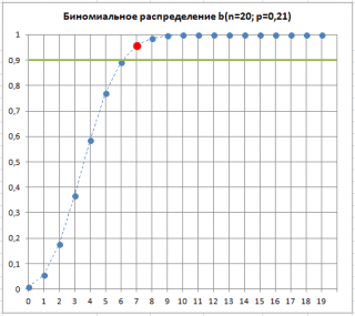
Thus, exceeding the threshold number of defective products in the sample may serve as a signal that the process has become upset and began to produce b about higher percentage of defective products.

Note: Prior to MS EXCEL 2010, EXCEL had a function CRITBINOM() , which is equivalent to BINOM.INV() . CRITBINOM() is left in MS EXCEL 2010 and higher for compatibility.

Relation of the Binomial distribution to other distributions

If the parameter nBinomial distribution tends to infinity and p tends to 0, then in this case Binomial distribution can be approximated. It is possible to formulate conditions when the approximation Poisson distribution works good:

• p(the less p and more n, the more accurate the approximation);
• p >0,9 (considering that q =1- p, calculations in this case must be performed using q(a X needs to be replaced with n - x). Therefore, the less q and more n, the more accurate the approximation).

At 0.110 Binomial distribution can be approximated.

In turn, Binomial distribution can serve as a good approximation when the population size is N Hypergeometric distribution much larger than the sample size n (i.e., N>>n or n/N You can read more about the relationship of the above distributions in the article. Examples of approximation are also given there, and conditions are explained when it is possible and with what accuracy.

ADVICE: You can read about other distributions of MS EXCEL in the article .

The binomial distribution is one of the most important probability distributions of discretely changing random variable. The binomial distribution is the probability distribution of a number m event AND in n mutually independent observations. Often an event AND called "success" of observation, and the opposite event - "failure", but this designation is very conditional.

Terms of the binomial distribution:

• carried out in total n trials in which the event AND may or may not occur;
• event AND in each of the trials can occur with the same probability p;
• the tests are mutually independent.

The probability that in n test event AND exactly m times, can be calculated using the Bernoulli formula:

where p- the probability of the event occurring AND;

q = 1 - p is the probability of the opposite event occurring.

Let's figure it out why the binomial distribution is related to the Bernoulli formula in the way described above . Event - the number of successes at n tests is divided into a number of options, in each of which success is achieved in m trials, and failure - in n - m tests. Consider one of these options - B1 . According to the rule of addition of probabilities, we multiply the probabilities of opposite events:

,

and if we denote q = 1 - p, then

.

The same probability will have any other option in which m success and n - m failures. The number of such options is equal to the number of ways in which it is possible from n test get m success.

The sum of the probabilities of all m event number AND(numbers from 0 to n) is equal to one:

where each term is a term of the Newton binomial. Therefore, the considered distribution is called the binomial distribution.

In practice, it is often necessary to calculate probabilities "at most m success in n tests" or "at least m success in n tests". For this, the following formulas are used.

The integral function, that is probability F(m) that in n observation event AND will come no more m once, can be calculated using the formula:

In turn probability F(≥m) that in n observation event AND come at least m once, is calculated by the formula:

Sometimes it is more convenient to calculate the probability that in n observation event AND will come no more m times, through the probability of the opposite event:

.

Which of the formulas to use depends on which of them contains fewer terms.

The characteristics of the binomial distribution are calculated using the following formulas .

Expected value: .

dispersion: .

Standard deviation: .

Binomial distribution and calculations in MS Excel

Binomial Distribution Probability P n ( m) and the value of the integral function F(m) can be calculated using the MS Excel function BINOM.DIST. The window for the corresponding calculation is shown below (click the left mouse button to enlarge).

MS Excel requires you to enter the following data:

• number of successes;
• number of tests;
• probability of success;
• integral - logical value: 0 - if you need to calculate the probability P n ( m) and 1 - if the probability F(m).

Example 1 The manager of the company summarized information on the number of cameras sold over the past 100 days. The table summarizes the information and calculated the probabilities that a certain number of cameras will be sold per day.

The day ends with a profit if 13 or more cameras are sold. The probability that the day will be worked out with a profit:

The probability that the day will be worked without profit:

Let the probability that the day is worked out with a profit be constant and equal to 0.61, and the number of cameras sold per day does not depend on the day. Then you can use the binomial distribution, where the event AND- the day will be worked out with profit, - without profit.

The probability that out of 6 days all will be worked out with a profit:

.

We get the same result using the MS Excel function BINOM.DIST (the value of the integral value is 0):

P 6 (6 ) = BINOM.DIST(6; 6; 0.61; 0) = 0.052.

The probability that out of 6 days 4 or more days will be worked with a profit:

where ,

,

Using the MS Excel function BINOM.DIST, we calculate the probability that out of 6 days no more than 3 days will be completed with a profit (the value of the integral value is 1):

P 6 (≤3 ) = BINOM.DIST(3, 6, 0.61, 1) = 0.435.

The probability that out of 6 days all will be worked out with losses:

,

We calculate the same indicator using the MS Excel function BINOM.DIST:

P 6 (0 ) = BINOM.DIST(0; 6; 0.61; 0) = 0.0035.

Solve the problem yourself and then see the solution

Example 2 An urn contains 2 white balls and 3 black ones. A ball is taken out of the urn, the color is set and put back. The attempt is repeated 5 times. The number of appearances of white balls is a discrete random variable X, distributed according to the binomial law. Compose the law of distribution of a random variable. Determine the mode, mathematical expectation and variance.

We continue to solve problems together

Example 3 From the courier service went to the objects n= 5 couriers. Each courier with a probability p= 0.3 is late for the object regardless of the others. Discrete random variable X- the number of late couriers. Construct a distribution series of this random variable. Find its mathematical expectation, variance, standard deviation. Find the probability that at least two couriers will be late for the objects.

In this and the next few notes, we will consider mathematical models of random events. Mathematical model is a mathematical expression representing a random variable. For discrete random variables, this mathematical expression is known as the distribution function.

If the problem allows you to explicitly write a mathematical expression representing a random variable, you can calculate the exact probability of any of its values. In this case, you can calculate and list all values ​​of the distribution function. In business, sociological and medical applications, there are various distributions of random variables. One of the most useful distributions is the binomial.

Binomial distribution is used to model situations characterized by the following features.

• The sample consists of a fixed number of elements n representing the outcome of some test.
• Each sample element belongs to one of two mutually exclusive categories that cover the entire sample space. Typically, these two categories are called success and failure.
• Probability of Success R is constant. Therefore, the probability of failure is 1 - p.
• The outcome (i.e. success or failure) of any trial is independent of the outcome of another trial. To ensure independence of outcomes, sample items are usually obtained using two different methods. Each sample element is randomly drawn from an infinite population without replacement or from a finite population with replacement.

Download note in or format, examples in format

The binomial distribution is used to estimate the number of successes in a sample consisting of n observations. Let's take ordering as an example. Saxon Company customers can use an interactive electronic form to place an order and send it to the company. Then the information system checks whether there are any errors in the orders, as well as incomplete or inaccurate information. Any order in doubt is flagged and included in the daily exception report. The data collected by the company indicates that the probability of errors in orders is 0.1. The company would like to know what is the probability of finding a certain number of erroneous orders in a given sample. For example, suppose customers have completed four electronic forms. What is the probability that all orders will be error-free? How to calculate this probability? By success, we mean an error when filling out the form, and we will consider all other outcomes as failure. Recall that we are interested in the number of erroneous orders in a given sample.

What outcomes can we observe? If the sample consists of four orders, one, two, three or all four may be wrong, in addition, all of them may be correctly filled. Can the random variable describing the number of incorrectly completed forms take on any other value? This is not possible because the number of incorrectly completed forms cannot exceed the sample size n or be negative. Thus, a random variable obeying the binomial distribution law takes values ​​from 0 to n.

Suppose that in a sample of four orders, the following outcomes are observed:

What is the probability of finding three erroneous orders in a sample of four orders, and in the specified order? Since preliminary studies have shown that the probability of an error in completing the form is 0.10, the probabilities of the above outcomes are calculated as follows:

Since the outcomes are independent of each other, the probability of the indicated sequence of outcomes is equal to: p*p*(1–p)*p = 0.1*0.1*0.9*0.1 = 0.0009. If it is necessary to calculate the number of choices X n elements, you should use the combination formula (1):

where n! \u003d n * (n -1) * (n - 2) * ... * 2 * 1 - factorial of the number n, and 0! = 1 and 1! = 1 by definition.

This expression is often referred to as . Thus, if n = 4 and X = 3, the number of sequences consisting of three elements extracted from a sample of size 4 is given by the following formula:

Therefore, the probability of finding three erroneous orders is calculated as follows:

(number of possible sequences) *
(probability of a particular sequence) = 4 * 0.0009 = 0.0036

Similarly, we can calculate the probability that among four orders one or two are wrong, as well as the probability that all orders are wrong or all are correct. However, as the sample size increases n it becomes more difficult to determine the probability of a particular sequence of outcomes. In this case, an appropriate mathematical model should be applied that describes the binomial distribution of the number of choices X objects from a sample containing n elements.

Binomial distribution

where P(X)- probability X success for a given sample size n and probability of success R, X = 0, 1, … n.

Pay attention to the fact that formula (2) is a formalization of intuitive conclusions. Random value X, obeying the binomial distribution, can take any integer value in the range from 0 to n. Work RX(1 - p)n – X is the probability of a particular sequence consisting of X successes in the sample, the size of which is equal to n. The value determines the number of possible combinations consisting of X success in n tests. Therefore, for a given number of trials n and probability of success R the probability of a sequence consisting of X success is equal to

P(X) = (number of possible sequences) * (probability of a particular sequence) =

Consider examples illustrating the application of formula (2).

1. Let's assume that the probability of filling out the form incorrectly is 0.1. What is the probability that three of the four completed forms will be wrong? Using formula (2), we obtain that the probability of finding three erroneous orders in a sample of four orders is equal to

2. Assume that the probability of incorrectly completing the form is 0.1. What is the probability that at least three out of four completed forms will be wrong? As shown in the previous example, the probability that three of the four completed forms will be wrong is 0.0036. To calculate the probability that at least three of the four completed forms will be incorrectly completed, you must add the probability that among the four completed forms three will be wrong, and the probability that among the four completed forms all will be wrong. The probability of the second event is

Thus, the probability that among the four completed forms at least three will be erroneous is equal to

P(X > 3) = P(X = 3) + P(X = 4) = 0.0036 + 0.0001 = 0.0037

3. Assume that the probability of incorrectly completing the form is 0.1. What is the probability that less than three out of four completed forms will be wrong? The probability of this event

P(X< 3) = P(X = 0) + P(X = 1) + P(X = 2)

Using formula (2), we calculate each of these probabilities:

Therefore, P(X< 3) = 0,6561 + 0,2916 + 0,0486 = 0,9963.

Probability P(X< 3) можно вычислить иначе. Для этого воспользуемся тем, что событие X < 3 является дополнительным по отношению к событию Х>3. Then P(X< 3) = 1 – Р(Х> 3) = 1 – 0,0037 = 0,9963.

As the sample size increases n calculations similar to those carried out in example 3 become difficult. To avoid these complications, many binomial probabilities are tabulated ahead of time. Some of these probabilities are shown in Fig. 1. For example, to get the probability that X= 2 at n= 4 and p= 0.1, you should extract from the table the number at the intersection of the line X= 2 and columns R = 0,1.

Rice. 1. Binomial probability at n = 4, X= 2 and R = 0,1

The binomial distribution can be calculated using the Excel function =BINOM.DIST() (Fig. 2), which has 4 parameters: the number of successes - X, number of trials (or sample size) – n, the probability of success is R, parameter integral, which takes the values ​​TRUE (in this case, the probability is calculated at least X events) or FALSE (in this case, the probability of exactly X events).

Rice. 2. Function parameters =BINOM.DIST()

For the above three examples, the calculations are shown in fig. 3 (see also Excel file). Each column contains one formula. The numbers show the answers to the examples of the corresponding number).

Rice. 3. Calculation of binomial distribution in Excel for n= 4 and p = 0,1

Properties of the binomial distribution

The binomial distribution depends on the parameters n and R. The binomial distribution can be either symmetric or asymmetric. If p = 0.05, the binomial distribution is symmetric regardless of the parameter value n. However, if p ≠ 0.05, the distribution becomes skewed. The closer the parameter value R to 0.05 and the larger the sample size n, the weaker is the asymmetry of the distribution. Thus, the distribution of the number of incorrectly completed forms is shifted to the right, since p= 0.1 (Fig. 4).

Rice. 4. Histogram of the binomial distribution for n= 4 and p = 0,1

Mathematical expectation of the binomial distribution is equal to the product of the sample size n on the likelihood of success R:

(3) M = E(X) =np

On average, with a sufficiently long series of tests in a sample of four orders, there may be p \u003d E (X) \u003d 4 x 0.1 \u003d 0.4 incorrectly completed forms.

Binomial distribution standard deviation

For example, the standard deviation of the number of incorrectly completed forms in an accounting information system is:

Materials from the book Levin et al. Statistics for managers are used. - M.: Williams, 2004. - p. 307–313

The theory of probability is invisibly present in our lives. We do not pay attention to it, but every event in our life has one or another probability. Given the huge number of possible scenarios, it becomes necessary for us to determine the most likely and least likely of them. It is most convenient to analyze such probabilistic data graphically. Distribution can help us with this. Binomial is one of the easiest and most accurate.

Before proceeding directly to mathematics and probability theory, let's figure out who was the first to come up with this type of distribution and what is the history of the development of the mathematical apparatus for this concept.

History

The concept of probability has been known since ancient times. However, ancient mathematicians did not attach much importance to it and were only able to lay the foundations for a theory that later became the theory of probability. They created some combinatorial methods that greatly helped those who later created and developed the theory itself.

In the second half of the seventeenth century, the formation of the basic concepts and methods of probability theory began. Definitions of random variables, methods for calculating the probability of simple and some complex independent and dependent events were introduced. Such an interest in random variables and probabilities was dictated by gambling: each person wanted to know what his chances of winning the game were.

The next step was the application of methods of mathematical analysis in probability theory. Eminent mathematicians such as Laplace, Gauss, Poisson and Bernoulli took up this task. It was they who advanced this area of ​​mathematics to a new level. It was James Bernoulli who discovered the binomial distribution law. By the way, as we will later find out, on the basis of this discovery, several more were made, which made it possible to create the law of normal distribution and many others.

Now, before we begin to describe the binomial distribution, we will refresh a little in the memory of the concepts of probability theory, probably already forgotten from the school bench.

Fundamentals of Probability Theory

We will consider such systems, as a result of which only two outcomes are possible: "success" and "failure". This is easy to understand with an example: we toss a coin, guessing that tails will fall out. The probabilities of each of the possible events (tails falling - "success", heads falling - "not success") are equal to 50 percent if the coin is perfectly balanced and there are no other factors that can affect the experiment.

It was the simplest event. But there are also complex systems in which sequential actions are performed, and the probabilities of the outcomes of these actions will differ. For example, consider the following system: in a box whose contents we cannot see, there are six absolutely identical balls, three pairs of blue, red and white colors. We have to get a few balls at random. Accordingly, by pulling out one of the white balls first, we will reduce by several times the probability that the next one we will also get a white ball. This happens because the number of objects in the system changes.

In the next section, we will look at more complex mathematical concepts that bring us close to what the words " normal distribution"," binomial distribution "and the like.

Elements of mathematical statistics

In statistics, which is one of the areas of application of the theory of probability, there are many examples where the data for analysis is not given explicitly. That is, not in numbers, but in the form of division according to characteristics, for example, according to gender. In order to apply a mathematical apparatus to such data and draw some conclusions from the results obtained, it is required to convert the initial data into a numerical format. As a rule, to implement this, a positive outcome is assigned a value of 1, and a negative one is assigned a value of 0. Thus, we obtain statistical data that can be analyzed using mathematical methods.

The next step in understanding what the binomial distribution of a random variable is is to determine the variance of the random variable and the mathematical expectation. We'll talk about this in the next section.

Expected value

In fact, understanding what mathematical expectation is is not difficult. Consider a system in which there are many different events with their own different probabilities. The mathematical expectation will be called the value, equal to the sum the products of the values ​​of these events (in the mathematical form we talked about in the last section) and the probability of their occurrence.

The mathematical expectation of the binomial distribution is calculated according to the same scheme: we take the value of a random variable, multiply it by the probability of a positive outcome, and then summarize the obtained data for all variables. It is very convenient to present these data graphically - this way the difference between the mathematical expectations of different values ​​is better perceived.

In the next section, we will tell you a little about a different concept - the variance of a random variable. It is also closely related to such a concept as the binomial probability distribution, and is its characteristic.

Binomial distribution variance

This value is closely related to the previous one and also characterizes the distribution of statistical data. It represents the mean square of deviations of values ​​from their mathematical expectation. That is, the variance of a random variable is the sum of the squared differences between the value of the random variable and its mathematical expectation multiplied by the probability of this event.

In general, this is all we need to know about variance in order to understand what the binomial probability distribution is. Now let's move on to our main topic. Namely, what lies behind such a seemingly rather complicated phrase "binomial distribution law".

Binomial distribution

Let's first understand why this distribution is binomial. It comes from the word "binom". You may have heard of Newton's binomial - a formula that can be used to expand the sum of any two numbers a and b to any non-negative power of n.

As you probably already guessed, Newton's binomial formula and the binomial distribution formula are almost the same formulas. With the only exception that the second has an applied value for specific quantities, and the first is only a general mathematical tool, the applications of which in practice can be different.

Distribution formulas

The binomial distribution function can be written as the sum of the following terms:

(n!/(n-k)!k!)*p k *q n-k

Here n is the number of independent random experiments, p is the number of successful outcomes, q is the number of unsuccessful outcomes, k is the number of the experiment (it can take values ​​from 0 to n),! - designation of a factorial, such a function of a number, the value of which is equal to the product of all the numbers going up to it (for example, for the number 4: 4!=1*2*3*4=24).

In addition, the binomial distribution function can be written as an incomplete beta function. However, this is already a more complex definition, which is used only when solving complex statistical problems.

The binomial distribution, examples of which we examined above, is one of the most simple species distributions in probability theory. There is also a normal distribution, which is a type of binomial distribution. It is the most commonly used, and the easiest to calculate. There is also a Bernoulli distribution, a Poisson distribution, a conditional distribution. All of them characterize graphically the areas of probability of a particular process under different conditions.

In the next section, we will consider aspects related to the application of this mathematical apparatus in real life. At first glance, of course, it seems that this is another mathematical thing, which, as usual, does not find application in real life, and is generally not needed by anyone except mathematicians themselves. However, this is not the case. After all, all types of distributions and their graphical representations were created solely for practical purposes, and not as a whim of scientists.

Application

By far the most important application of distributions is in statistics, where complex analysis of a multitude of data is required. As practice shows, very many data arrays have approximately the same distributions of values: the critical regions of very low and very high values, as a rule, contain fewer elements than the average values.

Analysis of large data arrays is required not only in statistics. It is indispensable, for example, in physical chemistry. In this science, it is used to determine many quantities that are associated with random vibrations and movements of atoms and molecules.

In the next section, we will understand how important it is to apply statistical concepts such as binomial distribution of a random variable in everyday life for you and me.

Why do I need it?

Many people ask themselves this question when it comes to mathematics. And by the way, mathematics is not in vain called the queen of sciences. It is the basis of physics, chemistry, biology, economics, and in each of these sciences, some kind of distribution is also used: whether it is a discrete binomial distribution or a normal one, it does not matter. And if we take a closer look at the world around us, we will see that mathematics is used everywhere: in everyday life, at work, and even human relationships can be presented in the form of statistical data and analyzed (this, by the way, is done by those who work in special organizations involved in the collection of information).

Now let's talk a little about what to do if you need to know much more on this topic than what we have outlined in this article.

The information that we have given in this article is far from complete. There are many nuances as to what form the distribution might take. The binomial distribution, as we have already found out, is one of the main types on which the whole mathematical statistics and probability theory.

If you become interested, or in connection with your work, you need to know much more on this topic, you will need to study the specialized literature. Start with a university course mathematical analysis and get there to the section of probability theory. Also knowledge in the field of series will be useful, because the binomial probability distribution is nothing more than a series of successive terms.

Conclusion

Before finishing the article, we would like to tell you one more interesting thing. It concerns directly the topic of our article and all mathematics in general.

Many people say that mathematics is a useless science, and nothing that they learned in school was useful to them. But knowledge is never superfluous, and if something is not useful to you in life, it means that you simply do not remember it. If you have knowledge, they can help you, but if you do not have them, then you cannot expect help from them.

So, we examined the concept of the binomial distribution and all the definitions associated with it and talked about how it is applied in our lives.